
Comparison- of the iterative approximations of the Colebrook-White equation
Here’s a review of other formulas and a mathematically exact formulation that is valid over the entire range of Re values
C. T. GOUDAR,* Bayer HealthCare, Berkeley, California, and J. R. SONNAD,
University of Oklahoma Health Sciences Center, Oklahoma City, Oklahoma
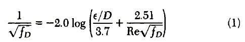
Friction factor estimation is a key component of piping system design and the Colebrook-White equation is typically the method of choice for computing turbulent flow friction factor in rough pipes:
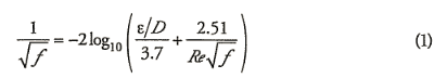
It relates the friction factor f implicitly to the pipe roughness, elD, and the Reynolds number, Re. Because of the implicit nature of Eq. I, graphical methods were originally proposed for f estimation1 and are still used today. While the visual representation in a graphical correlation is certainly appealing, accurate f determination is difficult and this approach is not suited for most current computer-based piping system design projects.
For computer implementation, iterative numerical methods such as the Newton-Raphson method2 can be used to determine f from Eq. 1. Ideally, these iterative calculations are not desirable, and in an attempt to simplify f estimation from Eq. I, several explicit approximations of f have been proposed.3-6 Accuracy of values determined from these correlations varies greatly and not all correlations are valid over a large Re range (typically 4,000 < Re < 108) to be universally applicable. Accuracy of the noniterative empirical correlations has been comprehensively evaluated7 and was found to be in the 1.42-28.23% range compared with 1% error for a simplifled form of a truly explicit representation of Eq. 1.
In addition to the noniterative correlations mentioned, several iterative approximations have also been proposed for Eq. 1_4- , 6 , 8 9
These are more complex functional relationships between f, e/D and Re but result in f values with higher accuracy. To completely eliminate need for empirical correlations, we have proposed an explicit, mathematically exact formulation of Eq. 1 that is valid over the entire range of Re values and results in highly accurate f values. 10, 11 Accuracy of a simplifled form of this formulation was presented earlier7 and in this study we present a comparison of two other forms of this formulation with the various iterative approximations of Eq. 1.
To completely eliminate need for empirical correlations, we have proposed an explicit, mathematically exact formulation of Eq. 1 that is valid over the entire range of Re values and results in highly accurate f values
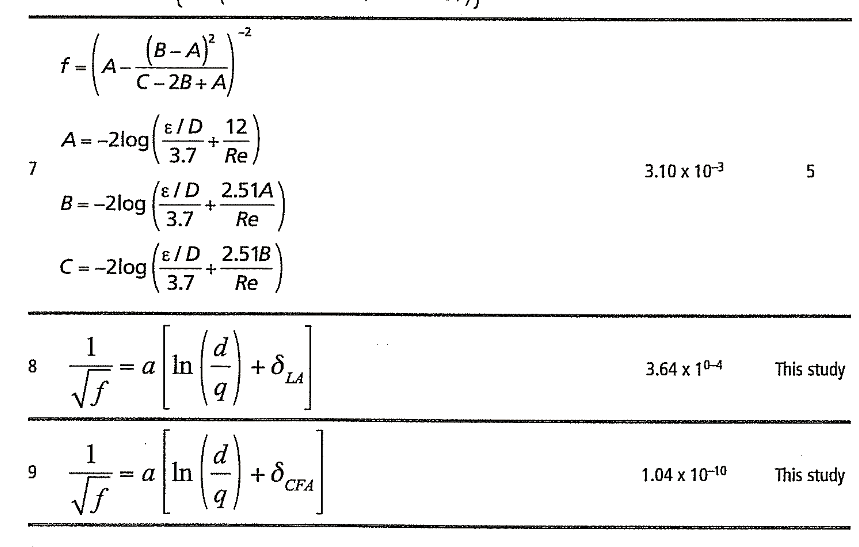
Details on the derivation of the explicit reformulation have been presented elsewhere11 and only the final equations are shown here. The friction factor f can be explicitly related to e/D and Re as:
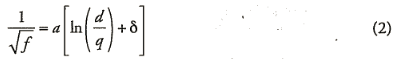
where:

Two different formulations are available for 8, the linear formulation, 8LA, and the continued fractions formulation, 8cFA and they vary in complexity and accuracy:

Thus, two versions of Eq. 2 are possible depending upon the choice of 8:

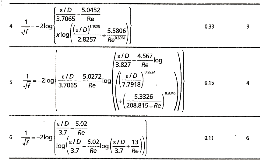
A comparison of the properties of various iterative empirical approximations of Eq. 1 is presented along with error in f’ estimates from Eqs. 4 and 5.
Comparison with empirical approximations. The accuracy of Eqs. 4 and 5 and the empirical iterative approximations of Eq. 1 were determined over a rectangular space of e/D and Re values. A set of 20 e/D values corresponding to those used by Moody1 were selected that spanned a range from 10-6 to 5 x 10⁻². For each e/D value 500 values of Re, distributed uniformly in the logarithmic space over 4,000 <Re< 108, were chosen. Accuracy of f values at these 10,000 points (20 x 500 grid of e/D and Re values) was determined by comparing them with those obtained from the highly accurate mathematically equivalent form.11
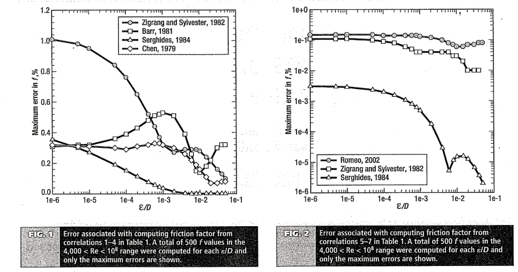
A total of 10,000 f values and their associated error were determined over the 20 x 500 grid of e/D and Re values, and the maximum error values are shown in Table 1. While not all Table 1 correlations are valid over the entire Re range (4,000 <Re< 108) , comparison was intentionally made over this extended range to reflect operational conditions. The maximum f error ranged from 1.01 to 3.10 x 10⁻³% with the Serghides correlation5 being the most accurate. Correlations 8 and 9, which are derived from an explicit mathematically equivalent representation of Eq. 1, were characterized by maximum f errors of 3.64 x 10⁻⁴ and 1.04 x 10– 10 %, both better than the best available iterative approximation.
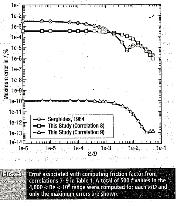
Accuracy of the correlations in Table 1 is shown in Figs. 1 and 2 where the maximum percentage f error is shown at varying e/D values. For each e/D value, 500 f values were determined at 500 logarithmically spaced Re values in the 4,000 <Re< 108 range and the maximum values are shown in Figs. 1 and 2. The Serghides equation (correlation 7) with a maximum error of 3.1 x 10⁻³% is the best available empirical approximation. Fig. 3 shows a comparison of f error profiles for the Serghides equation with those from Eqs. 4 and 5. Maximum error from Eqs. 4 and 5 were 3.64 x10⁻⁴ and 1.04 x 10– 10%, respectively, and this improved accuracy is reflected in Fig. 3.


LITERATURE CITED
1 Moody, L. F. « Friction factors for pipe flow, » Trans. ASME 66, 1944, pp. 671-684.
2 Press, W. H., et al., Numerical Recipes in FORTRAN: The an of scientific computing, New York Cambridge University Press, 1992.
3 Gregory, G. A. and M. Fogarasi, « Alternate to standard friction factor equation, » Oil and Gas Journal 1985, pp. 120-127.
4 Romeo, E., C. Royo, and A. Monzon, « Improved explicit equations for estimation of the friction factor in rough and smooth pipes, » Chem Eng. 86, 2002, pp. 369-374.
5 Serghidcs, T. K, « Estimate friction factor accu-rately, » Chem. Eng. 91, 1984, pp. 63-64.
6 Zigrang, D. J., and N. D. Sylvester, « Explicit approximations to the solution of Colebrook’s friction faaor equation, » AIChE J. 28, 1982, pp. 514-515.
7 Goudar, C. T. and J. R. Sonnad, « Explicit friction factor correlation for turbulent flow in rough pipe, » Hydrocarbon Processing 86, 2007, pp. 103-105.
8 Barr, D. I. H.; « Solutions of the Colebrook-White function for resistance to uniform turbulent flow, » Proc. Inst. Civil big. 71, 1981, pp. 529-535.
9 Chen, N. H., « An explicit equation for friction factor in pipe, » Ind Eng. Chem. Fund. 18, 1979, pp. 296-297.
10 Sonnad, J. IL and C. T. Goudar, « Turbulent flow friction factor calculation using a mathematically-exact alternative to the Colebrook-White equation, J. Hydr. Eng. 132, 2006, pp. 863-867.
11 Sonnad, J. R. and C. T. Goudar, « Explicit reformulation of the Colebrook-White equation for turbulent flow friction factor calculation, » Intl Eng. Chem. Res. 46, 2007, pp, 2593-2600.
Friction Factors for Pipe Flow
Br LEWIS F. MOODY,’ PRINCETON, N. J.
The object of this paper is to furnish the engineer with a simple means of estimating the friction factors to be used in computing the loss of head in clean new pipes and in closed conduits running full with steady flow. The modern developments in the application of theoretical hydrodynamics to the fluid-friction problem are impressive, and e scattered through an extensive literature. This paper is not intended as a critical survey of this wide field. .For a concise review, Professor Bakhmeteff’s (1)2 small book on the mechanics of fluid flow is an excellent reference. Prandtl and Tietjens (2) and Rouse (3) have also made notable contributions to the subject. The author does not claim to offer anything particularly new or original, his aim merely being to embody the now accepted conclusions in convenient form for engineering use.
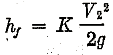
In the present pipe-flow study, the friction factor, denoted by f in the accompanying charts, is the coefficient in the Darcy formula

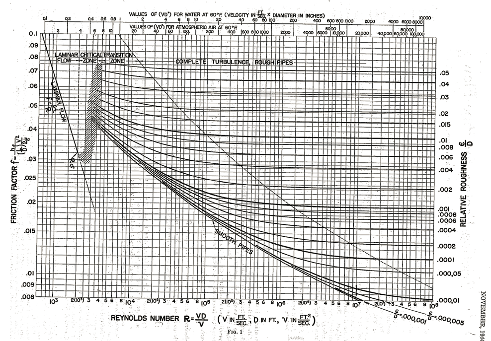
in which hf is the loss of head in friction, in feet of fluid column of the fluid flowing; L and D the length and internal diameter of the pipe-in.-feet; V the mean velocity of flow in feet per second; and g the acceleration of gravity in feet per second per second (mean Value taken as 32.16). The factor f is a dimensionless quantity, and at ordinary velocities is a function of two, and only two, other dimensionless quantities, the relative roughness of the surface, e/D (e being a linear quantity in feet representative of the absolute roughness), and the Reynolds number R = VD /v (v being the coefficient of kinematic viscosity of the fluid in square feet per second). Fig. 1 gives numerical values of f as a function of e/D and R.
Ten years ago R. J. S. Pigott (4) published a chart for the same friction factor, using the same co-ordinates as in ‘Fig. 1 of this paper. His chart has proved to be most useful and practical and has been reproduced in a number of texts (5). The Pigott chart was based upon an analysis of some 10,000 experiments from various sources (6), but did not have the benefit, in plotting or fairing the curves, of later developments in functional forms of the curves.
In the same year Nikuradse (7) published his experiments on artificially roughened pipes. Based upon the tests of Nikuradse and others, von Karman (8) and Prandtl (9) developed their theoretical analyses of pipe flow and gave us suitable formulas with numerical constants for the case of perfectly smooth pipes or those in which the irregularities are small compared to the thickness of the laminar boundary layer, and for the case of rough pipes where the roughnesses protrude sufficiently to break up the laminar layer, and the flow becomes completely turbulen
i Professor, Hydraulic Engineering, Princeton University. Mem. A.S.M.E.
2 Numbers in parentheses refer to the Bibliography at the end of the paper.
Contributed by the Hydraulic Division and presented at the Semi-Annual Meeting, Pittsburgh, Pa., June 19-22, 1944, of THE
MEIBRICAN SOCIETY OF MECHANICAL ENGINEERS
Nom: Statements and opinions advanced in papers are to be understood as individual expressions of their authors and not those of the Society.
The analysis did not, however, cover the entire field but left a gap, namely; the transition zone between smooth and rough pipes, the region of incomplete turbulence. Attempts to fill this gap by the use of Nikuradse’s results for artificial roughness produced by closely packed sand grains, were not adequate, since the results were clearly at variance from actual experience for ordinary surfaces encountered in practice. Nikuradse’s curves showed a sharp drop followed by a peculiar reverse curve, not observed with commercial surfaces, and nowhere suggested by the Pigott chart based on many tests.
Recently Colebrook (11), in collaboration with C. M. White; developed a function which gives a practical form of transition curve to bridge the gap. This function agrees with the two extremes of roughness and gives values in very satisfactory agreement with actual measurements on most forms of commercial piping and usual pipe surfaces. Rouse (12) has shown that it is a reasonable and practically adequate solution and has plotted a chart based upon it. In order to simplify the plotting, Rouse adopted co-ordinates inconvenient for ordinary engineering use, since f is implicit in both co-ordinates, and R values are represented by curved co-ordinates, so that interpolation is troublesome.
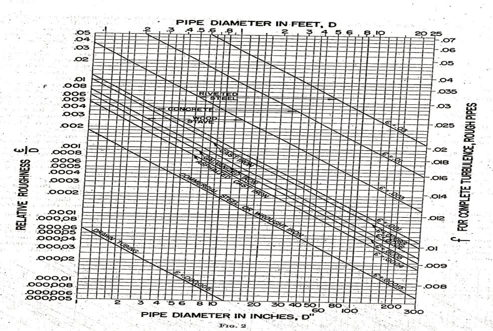
The author has drawn up a new chart, Fig. 1, in the more conventional form used by Pigott, taking advantage of the functional relationships established in recent years. Curves of f versus R are plotted to logarithmic scales for various constant values of relative roughness (e/D); and to permit easy selection of e/D, an accompanying chart, Fig. 2, is given from which e/D can be read for any size of pipe of a given type of surface.
In order to find the friction loss in a pipe, the procedure is as follows: Find the appropriate (e/D) from Fig. 2, then follow the corresponding line, thus identified, in Fig. 1, to the value of the Reynolds number R corresponding to the velocity of flow. The factor f is thus found, for use in the Darcy formula

In Fig. 2, the scales at the top and bottom give values of the diameter in both feet and inches. Fig. 1 involves only dimensionless quantities and is applicable in any system of units.
To facilitate the calculation of R, auxiliary scales are shown at the top of Fig. 1, giving values of the product (V.D ») for two fluids, i.e., water and atmospheric air, at 60 F. (D » is the inside diameter in inches.) As a further auxiliary, Fig.3 is given, from Which R can be quickly found for water at ordinary temperatures, for any size of pipe and mean velocity V. Dashed lines on this chart have been added giving values of the discharge or quantity of fluid flowing, Q = AV, expressed in both -cubic feet per second and in U. S. gallons per minute.
3 Rouse, reference (3), p. 250; and Powell, reference (10), p. 174.
For other fluids, the kinematic viscosity v may be found from Fig. 4, which with. Prof. R. L. Daugherty’s kind permission has been reproduced to enable R to be quickly found for various fluids, Fig. 4 includes an auxiliary diagram constructed by Dr. G. F. Wislicenus, which gives R for various values of the product VD » shown by the diagonal lines. – For any value of v in the left-hand diagram, by following a horizontal line to the appropriate diagonal at the right, the corresponding R may be read at the top of the auxiliary graph.
Over a large part of Fig. 1, an approximate figure for R is sufficient, since f varies only slowly with changes in R; and in the rough-pipe zone f is independent of R. From the last consideration, it becomes possible to show, in the right-hand margin of Fig. 2, values of f for rough pipes and complete turbulence.
Reference (13) and reference (5).
If it is seen that the conditions of any problem clearly fall in the zone of complete turbulence above and to the right of the dashed line in Fig. 1, then Fig. 2 will give the value of f directly without further reference to the other charts.
ILLUSTRATION OF USE OF CHARTS
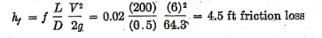
Example 1: To estimate the loss of head in 200 ft of 6-in. asphalted cast-iron pipe carrying water with a mean velocity of 6 fps: In Fig. 2, for 6 in. diam (bottom. scale), the diagonal for « asphalted cast iron » gives e/D= 0.0008 (left-hand margin). In Fig. 3, for 6 in. diam (left-hand margin), the diagonal for V = 6 fps gives R = 2.5 (105) (bottom scale) (or, instead of using Fig. 3, compute VD » = 6 X 6 = 36). In Fig. 1, locate from the right-hand margin the curve for e/D= 0.0008 and follow this curve to a point above R = 2.5 (105) on the bottom scale (or below VD » = 36 on the top scale). This point gives f = 0.02 (left-hand margin); then:
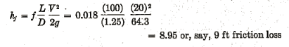
Example 2: To estimate the loss of head per 100 ft in a 15-in. new cast-iron pipe, carrying water with a mean velocity of 20 fps: In Fig. 2, for 15 in. dim (bottom scale), the diagonal for « cast iron » gives e/D= 0.0007 (left-hand margin). In Fig. 3, for 15 in. diam (left-hand margin), the diagonal for V = 20 fps gives R = 2 (106) (or, instead of using Fig. 3, compute VD »= 20 X 15= 300). In Fig. 1, the curve for e/D= 0.0007 (interpolating between 0.0006 and 0.0008, right-hand margin), at a point above R = 2 (106) (bottom scale) (or below VD » = 300, top scale) gives f = 0.018 (left-hand margin). In this case the point on Fig. 1 falls just on the boundary of the region of « complete turbulence; rough pipes. » Here R or VD » need only be approximated sufficiently to see that the point falls in the complete turbulence region, and f can then be found directly from the right-hand margin in Fig. 2 without further reference to Fig. 1; then
It must be recognized that any high degree of accuracy in determining f is not to be expected. With smooth tubing, it is true, good degrees of accuracy are obtainable; a probable variation in f within about ±5 per cent (14), and for commercial steel and wrought-iron piping, a variation within about ±10 per cent. But, in the transition and rough-pipe regions, we lack the primary and obvious essential, a technique for measuring the roughness of a pipe mechanically. Until such a technique is developed, we have to get along with descriptive terms to specify the roughness; and naturally this leaves much latitude. The lines in Fig. 2 might be more graphically represented by broad bands rather than single lines, but this is not practical due to overlapping.
Even with this handicap, however, fairly reasonable estimates of friction loss can be made, and, fortunately, engineering problems rarely require more than this. It will be noted from the charts that a wide variation in estimating the roughness affects f to a much smaller degree. In the rough-pipe region, for the reasons just explained, the values of f cannot be relied upon within a range of the order of at least 10 per cent.
The charts apply only to new and clean piping, since the rapidity of deterioration with age, dependent upon the quality of the water or fluid and that of the pipe material, can only be guessed in most cases; and in addition to the variation in roughness there may be, in old piping, an appreciable reduction in effective diameter, making an estimate of performance speculative.
Although we have no accepted method of direct measurement of the roughness, in any case where we have a sample of pipe of the same surface texture available for test in the laboratory or in the field, then from a test of such a pipe in any size we can, by aid of the charts, find the absolute roughness corresponding to its performance. Thus we have a means for measuring the Toughness hydraulically. The scale of the absolute roughness e used in plotting the charts is arbitrary, based upon the sand-grain diameters of Nikuradse’s experiments.
The field covered by Fig. 1 divides itself into four areas representing distinct flow characteristics. The first is the region of laminar flow, up to the critical Reynolds number of 2000. Here the flow is fully stabilized under the control of viscous forces which damp out turbulence, permitting a completely rational solution. The values off are here given by a single curve, f = 64/R independent of roughness, representing the Hagen -Poiseuille law.
Between Reynolds numbers of 2000 and 3000 or 4000, the conditions depend upon the initial turbulence due to such extraneous factors as sudden changes in section, obstructions, or a sharp-edged entrance corner prior to the reach of pipe considered;


and the conditions are probably also affected by pressure waves initiating instability. This region has been called a critical zone, and the indefiniteness of behavior in this region has been indicated by a hatched area without definite f lines. The minimum for f values is the dotted continuation of the laminar-flow line, corresponding to very smooth and steady initial flow. When there is distinct turbulence in the entering fluid, the flow in the’ critical zone is likely to be pulsating (2) rather than steady. The effects of strong initial turbulence may even extend into the laminar-flow zone, raising the f values somewhat, as far as to a Reynolds number of about 1200. Above a Reynolds number of 3000 or 4000, conditions again become reasonably determinate. Here we find two regions, namely, the transition zone and the rough-pipe zone. The transition zone extends upward from the line for perfectly smooth pipes, for which the equation is

(Karman., Prandtl, Nikuradse) to the dashed line indicating its upper limit, plotted
from the relation

(following the corresponding line in Rouse’s chart, reference 12).
In the transition zone the curves follow the Colebrook function.

These curves are asymptotic at one end to the smooth pipe line and at the other to the horizontal lines of the rough-pipe zone. Actually, the curves converge rapidly to these limits, merging with the smooth pipe line at the left, and at the right, beyond the dashed line, becoming indistinguishable from the constant f lines for rough pipe.
THE COLEBROOK FUNCTION
The basis of the Colebrook function may be briefly outlined. Von Kerman had shown that, for completely turbulent flow in rough pipes, the expression

is equal to a constant (1.74), or, as expressed by Colebrook,

is equal to-zero. In the transition region of incomplete turbulence von Karman’s expression is not equal to a constant but to some function of the ratio of the size of the roughnesses to the thickness of the laminar boundary layer. Accordingly, Nikuradse had represented his experimental results on artificially roughened pipes by plotting
versus

in which

is the laminar layer thickness. By this method of plotting, the results for all types of flow and degrees of roughness were shown to fall on a single curve. Using logarithmic scales, the smooth-pipe curve becomes an inclined straight line, and the rough-pipe curves merge in a single horizontal line.
Colebrook (11), using equivalent co-ordinates,5 plotted in his Fig. 1, here reproduced as Fig. 5, the results of many groups of tests on various types of commercial pipe surfaces. He found that each class of commercial pipe gave a curve of the same form, and while these curves are quite different from Nikuradse’s sand-grain results, they agree closely with each other and with a curve representing his transition function.
t’e/a may be expressed in alternative forms as proportional to R-Vf in which r = D/2, k = e; or to p V*k in which V* = ‘ r/k ‘2 . Ti’ To being the shearing stress at the pipe wall, p the mass density of the fluid andµ its absolute or dynamic viscosity.


Rouse « (12), also using equivalent co-ordinates, has plotted in his Fig. 6, here reproduced as Fig. 6, a large number of points each of which represents a series of tests on a given size of commercial pipe, together with the Colebrook curve. As he points out, the deviation of the points from the Colebrook curve « is evidently not much greater than the experimental scatter of the individual measurements in any one series ».
When the thickness of the laminar layer, which decreases with increasing Reynolds number, becomes so small, compared to the surface irregularities, that the laminar flow is broken up into turbulence, the flow conditions pass over into the zone of « rough pipes, » with complete turbulence established practically throughout the flow. Viscous forces then become negligible compared to inertia forces, and f ceases to be a function of the Reynolds number and depends only upon the relative roughness; giving horizontal lines of constant f in the chart. These lines agree with the von Karman rough-pipe formula:

Since f depends upon the relative roughness, the ratio of the absolute roughness to the pipe diameter, even a fairly rough surface in a very large pipe gives a small relative roughness. Thus Colebrook plots the results obtained on the penstocks of the Ontario Power Company, where metal forms and specially laid concrete produced a very smooth example of concrete surface. This in combination with the large diameter gave a relative roughness comparable to drawn brass tubing, with f values falling practically on the « smooth pipe » line of Fig. 1. Such specially fabricated, welded-steel pipe lines as those of the Colorado aqueduct system would probably give values along the same curve.
On the other hand, at very high velocities in drawn tubing of small diameter, even the small absolute roughness is sufficient to break up the laminar boundary layer, and the tubing becomes in effect a « rough pipe. » Very few experiments have carried the velocities and Reynolds numbers high enough to permit a close estimate of e for drawn brass, copper, or similar tubing; but by applying the Colebrook function to the available data (14, 15), for the smoothest surfaces reported upon, e was estimated as of the order of 0.000005; and a line corresponding to this value has been drawn in Fig. 2, serving as a minimum limit for surfaces likely to be encountered in practice.
PIPE FRICTION FACTORS APPLIED TO OPEN-CHANNEL FLOW
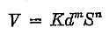
Pipe friction factors have sometimes been applied to open-channel flow, and more commonly the friction losses in large pipes and other closed conduits have been computed from open-channel formulas. The Chezy formula for open channels is

in which V is the mean velocity; m the hydraulic mean depth or « hydraulic radius, » the sectional area divided by the wetted perimeter; S the slope, the loss of head divided by length of channel, and C a coefficient. The Chezy formula is equivalent to the Darcy formula for pipes, the Chezy coefficient C being convertible into f by the relation f= 8g/C2. It should be considered, however, that the Chezy coefficients have been derived principally from observations on relatively wide and shallow channels of large area and rough bottoms, far from circular in shape, and that they involve a free water surface not present in closed conduits, so that; even when the flow is uniform, the problem is highly complex. Consequently, such formulas as Manning’s are recommended for open channels in preference to the use of values of C derived from the pipe friction factors.
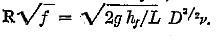
Open channels dealt with in engineering practice are usually rough surfaced and of large cross section, corresponding to large Reynolds numbers and falling in the zone of complete turbulence, so that the friction factors are practically independent of Reynolds number. The presence of a free surface, however, with surface waves or disturbances, introduces a consideration not involved in closed-conduit flow. It is therefore the author’s view that while, for open channels, we can drop the Reynolds number as an index of performance, we should replace it by a new criterion, the Froude number relating the velocity head and depth, which can be expressed as

or more strictly

in which

denotes the average depth or, sectional area divided by the surface breadth; the latter form representing the .ratio of mean velocity to the gravitational critical velocity or velocity of propagation of surface waves.
This proposed criterion defines whether the flow falls in the « tranquil, » « shooting, » or critical state. The neglect of this factor may at least partially account for inconsistencies between various open-channel formulas, and between open-channel and pipe-friction formulas, and casts particular doubt on accepted formulas for open-channel friction in the critical or shooting-flow regions, These considerations suggest the plotting of open-channel friction factors as a function of the relative roughness and the Froude number, in similar manner to the plotting off as a function of the relative roughness and the Reynolds number for closed conduits.
For the foregoing reasons, Fig. 1 is not recommended with much confidence for general application to open channels, for which a formula such as Manning’s better represents the available information. The charts can however be applied, at least as an approximation, to noncircular closed conduits of not too eccentric a form or not too different from a circular section, by using an equivalent diameter

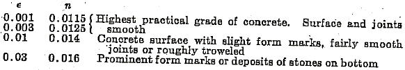
Since civil engineers usually classify surface roughness by the Kutter and Manning roughness factor n, it would be helpful in selecting a value of e for such variable surfaces as concrete, if we could correlate e and n. P. Panagos6 has applied the Colebrook function to the test data collected by Scobey (16) and finds the following values of e corresponding to the Rutter n ratings given by Scobey, which may be at least tentatively utilized:
Kutter n 0.0105 0.011 0.012 0.013 0.014 0.015 0.016
Absolute roughness e 0.00015 0.0005 0.002 0.005 0.011 0.02 0.03
Accordingly, on the basis of Scobey’s data the lines given in Fig. 2 for concrete may be somewhat more definitely described as follows:
Although the curves in Fig. 1 are plotted from definite functional forms which can be accepted with some confidence within the degree of accuracy required in engineering use, further information will be welcomed which would improve the location and definition of the lines in Fig. 2, or which would add new lines for other materials. Any tests of friction head in pipe of any material can be applied to Fig, 1, and corresponding points can be readily located in Fig. 2. A 45-deg line through a point so located can then be added to Fig. 2, to represent a particular kind of pipe surface.
ACKNOWLEDGMENT
For helpful suggestions and assistance, the author is particularly indebted to Prof. B. A. Bakhmeteff, Mr. Ralph Watson, Dr. G. F. Wislicenus, Dr, A. T. Ippen; and to Mr. P. Panagos for collecting data and numerical checking.
BIBLIOGRAPHY
1 « The Mechanics of Turbulent Flow, »-by B. A. Bakhmeteff, Princeton University Press, 1936.
2 « Applied Hydro- and Aeromechanics, » by L. Prandtl and 0. G. Tietjens, Engineering Societies MOnographs, McGraw-Hill Book Company, Inc., New York, N. Y., 1934.
3 « Fluid Mechanics for Hydraulic Engineers, » by H. Rouse, Engineering Societies Monographs, McGraw-Hill Book. Company, Inc., New York, N. Y., 1938.
4 « The Flow of Fluids in Closed Conduits, » by R. J. S. Pigott, Mechanical Engineering, vol. 55, 1933, pp. 497-501, 515.
5 « Hydraulics, » by R. L. Daugherty, McGraw-Hill Book Company, Inc., New York, N. Y., 1937.
6 « A Study of the Data on the Flow of Fluid in-Pipes, » by E. Keinler, Trans. A.S.M.E., vol. 55, 1933, paper Hyd-55-2, pp. 7-32.
7 « Stromungsgesetze in Rauhen Rohren, » by J. Nikuradse, V.D.Z.Forsch,ungsheft 361, Berlin, 1933, pp. 1-22.
8 « Mechanische Ihnlichkeit and Turbulenz, » by Th. von ICArman, Nachrichten von der Gesellschaft der Wissenschaften Fu Gottingen, 1930, Fachgruppe 1, Mathematik, no. 5, pp. 58-76. (« Mechanical Similitude and Turbulence, » Tech. Mem. NA.C.A.., no. 611, 1931.)
9 « Neuere Ergebnisse der Turbulenzforschung, » by L. Prandtl, Zeitschrift des Vereines deutscher Ingenieure, vol. 77, 1933, pp. 105-114.
10 « Mechanics of Liquids, » by R. W. Powell, the MacMillan Company, New York, N. Y., 1940.
11 « Turbulent Flow in Pipes, With Particular Reference to the Transition Region Between the Smooth and Rough Pipe Laws, » by C. F. Colebrook, Journal of the Institution of Civil Engineers (London, England), vol. 11, 1938-1939, pp. 133-156.
12 « Evaluation of Boundary Roughness, » by H. Rouse, Proceedings Second Hydraulic Conference, University of Iowa Bulletin 27, 1943.
13 « Some Physical Properties of Water and Other Fluids, » by R. L. Daugherty, Trans. A.S.M.E., vol. 57, 1935, pp. 193-196..
14 « The Friction Factors for Clean Round Pipes, » by T. B. Drew, E. C. Soo, and W. H. McAdams, Trans. American Institute of Chemical Engineers, vol. 28, 1932, pp. 56-72.
15 « Experiments Upon. the Flow of Water in Pipes and Pipe Fittings, » by J. R. Freeman, published by THE AMERICAN SOCIETY or MECHANICAL ENGINEERS, 1941.
16 « The Flow of Water in Concrete Pipe, » by F. C. Scobey, Bulletin 852, U. S. Department of Agriculture, October, 1920.
6 Assistant in Mechanical Engineering, Princeton University, Princeton, N. J.
Discussion
R. L. DAUGHERTY.? The writer has nothing but commendation for this excellent paper. The author has presented the latest theory combined with the available experimental data in a manner which makes it more convenient for use than has been the case heretofore. His evaluation of relative roughness for different types and sizes of pipes is a step forward.
While this paper deals primarily with pipe friction it is interesting to note the suggestions made concerning the treatment of the flow in open channels. The latter has not been given the attention from the standpoint of rational analysis that has been devoted in the past to pipes. It is to be hoped that developments in this field may be made along the lines suggested by the author.
The author calls attention to the well-known fact that in the transition zone the Nikuradse curves for his artificial sand-grain roughness are quite different from those obtained with commercial pipes. The writer would like to know if the author has any explanation to offer for this marked difference.
C. W. HUBBARD.B This paper is of interest to engineers who must estimate fluid-friction loss closely for certain types of problems. Ordinarily the Manning type of formula is preferred, since the roughness value may be determined from the Lype of surface of the wall as contrasted to the Darcy formula where the roughness coefficient varies with the size of pipe and is difficult to estimate. The author’s Fig. 2 allows a quantitative wall roughness estimated from the type of wall to be used.
During some recent tests made to select a protective paint for steel which would also have a low friction loss, it was found that several coatings, particularly those consisting of certain bitumastic constituents which required them to be applied thickly to the wall, gave low flow-resistance values. The tests, made in 3-in. pipes, which were split longitudinally to allow proper application of the coating, showed roughness values of the order of those obtained with drawn-brass tubing. However, the appearance of the coating was not as smooth as drawn tubing. The writer had previously experienced this effect with similar coatings. There seems to be little published material on the friction loss produced by various protective paints and coatings on pipe walls, particularly on small pipes when the flow is likely to occur in the transition range where the friction loss is dependent upon Reynolds number. Apparently the roughness of such surfaces is of the wavy Gype which cannot be evaluated on the same basis as the same magnitude of roughness which is of the granular type.
A. T. IPPEN.9 The author has ably satisfied the object of his paper stated in the beginning with an extremely timely and practical summary of the latest information available on pipe friction. Academic research in this field over the last 30 years conducted on a fundamental basis has finally yielded a satisfactory explanation of the nature of the laws of pipe friction and has cleared up the concepts of energy dissipation in conduits and channels.
? Professor of Mechanical. Engineering, California Institute of -Technology, Pasadena, Calif.
Lieutenant Commander, U.S.N.R. Mena. A.S.M.E.
Assistant Professor, Hydraulic Laboratory, Lehigh University, Bethlehem, Pa.
The evidence for the adoption of the methods for, determining the pipe friction factor as presented by Colebrook is rather astonishing. Some experiences in this connection may be contributed here. The writer has computed two comprehensive sets of data on, pipe friction, one by John R. Freeman and another by L. H. Kessler. The former completed his experiments during the years 1889 to 1893 and his data were published by this Society in a special volume (15)10 in 1941. The second set of data was obtained from pipe friction experiments at the Wisconsin Experimental Station, the results of which were published in 1935. Both experimenters performed tests on 1/4 in- to 8 in diameter wrought-iron pipes in new condition covering the maximum range in Reynolds numbers possible under their experimental conditions. After plotting these results every one of their rails shows essentially the f versus R curve indicated by Colebrook and ‘e values calculated for all the various sizes come out very close to the average value stated for wrought-iron pipe in the present paper. It must be remembered that Kessler’s data were obtained 40 years after those of Freeman and that it can hardly be assumed that manufacturing processes remained identical during that period.
Another fact of importance to the practical engineer from this analysis of Freeman’s and Kessler’s data is worth mentioning. Rouse and Moody in their f versus R curves terminate the transition range from smooth- to rough-pipe flow along a line corresponding to a ratio of absolute roughness e to the laminar boundary layer thickness a of 6.08. Kessler’s and Freeman’s data do not give a single value that high in all their runs; their highest values obtained were about = 2.5. Under practical conditions of use therefore the flow of water in pipes occurs well in the transition range from smooth-to rough-pipe flow.
This fact easily explains why a final solution of the pipe friction problem was possible only after the concepts of « smooth-pipe » and « rough-pipe » flow had been established separately. While Nikuradse’s results on uniformly sand-coated pipe were helpful in this respect, they also resulted in more complicated transition curves than are obtained from tests with the statistical roughness patterns encountered of the most commercial pipe surfaces. The Colebrook universal function seems to fit the better in this transition range; the more, the roughness irregularities are statistically distributed as fax as size and shape are Concerned and vice-versa, the more regular the size and pattern of the irregularities the closer Nikuradse’s transition curves are approached, where finally the critical velocity for all roughness bodies is the same in the ideal case of completely uniform size.
The familiar functions for the pipe friction factor f may be written in the following form
1, Numbers in parentheses throughout the discussion refer to the Bibliography at the end of the author’s paper.
According to Colebrook, Equations, [1] and [2] are combined into the following universal function

This function reverts to either Equation [1] or Equation [2], if either the influence of the relative roughness disappears or when the viscous influence becomes insignificant. By use of Equation [3], the Colebrook function may be written in the alternative form
This equation clearly brings out the dependence of the pipe friction phenomena upon the thickness of the laminar boundary layer, i.e., on the viscosity of the fluid. It will be found in practical calculations that this influence is very seldom absent. The proposed ultimate value of
is equivalent to a value of

of 6.08.
It is evident that aging of pipes under varying conditions of use will result in new values of absolute roughness which at present are not easily’ predicted. From experiments on galvanized steel pipe of 4 in. diam at the Hydraulic Laboratory of Lehigh University, an initial average value of e = 0.00045 ft was obtained. This value of e was doubled within 3 years as a result of the change in surface conditions with aging under moderate conditions of use. It must be remembered here that this change in e represents only about a 20 per cent increase in the Darcy-Weisbach factor f, since the e value is a much more sensitive indicator of pipe roughness than the factor f.
In conclusion, it may be hoped that this paper will bring the general adoption of this relatively easy and reliable method of determining pipe friction and thereby establish a standard procedure in practice which is based upon sound analytical and experimental evidence.
W. S. PARDoE.11 In the following tests on pipes of various diameters and materials, the exponent n in the exponential formula,
varied from 0.535 to 0.546, thus checking Williams’ and Hazen’s formula

very closely.
The maximum value of R was about 1,250,000 for 8-in. Neoprene dock-loading hose (very smooth) which is much below the « complete turbulence zone. » The tests included:
6-in. halite cement-asbestos pipe (predecessor of Transite)
4-in. Ruberoid cement-asbestos extruded pipe
4-in. fiber conduit
6-in, and 8-in. Neoprene dock-loading hose for E. I. du Pont de Nemours
2-in. to 12-in. steel pipe
8-in. rubber dock-loading hose with 1-in. X 1/8-in. helical metal band on inside
In no case except the last did the exponent n show even a tendency of decreasing, let alone approaching a value of 0.5 or complete turbulence. This must be due to the smoothness of the materials and the low value of Reynolds number. In the last case, the values of f did show a tendency to become constant, the value of e/D being quite large.
11 Department of Civil Engineering, University of Pennsylvania, Philadelphia. Pa,
The writer has not conducted a sufficient number of tests on pipes and is far from a pundit on this subject. At some time in the future, he will attempt to -work into the « complete turbulence zone, » if such there is, even if he must use a bit of 4-in. turberculated cast-iron pipe.
Mr. Pigott in his discussion has mentioned my insistence on the fact that the coefficients of Venturi meters become constant. This coefficient may be approximated by the formula
in which if β is the diameter ratio d2/dl and K is the coefficient of loss in
The value of K on the flat part of tests of 85 cast-iron Venturi meters approximates
As the absolute roughness is constant, the proportional roughness varies inversely as the diameter or the coefficient increases with the diameter. The tests ran to quite high values of Reynolds number in terms of

thus indicating there is such a thing as complete turbulence. Solving the foregoing expression

Hence a constant value of c gives a constant K, or nf varies as V2.
This is of course arguing from the writer’s experience with Venturi meters to make up for his lack of adequate experimental knowledge of the subject under discussion.
Professor Moody says f is a function of « two and only two », dimensionless quantities

and

The writer has found in his work on Venturi meters a variation of over 1/2 per cent, due to the effect of the ambient temperature.12
As a variation of 1/2 per cent in c requires a variation of 25 per cent in k it seems to the writer the effect of a difference of temperature of 20 deg F on f at low value of R might be considerable. This effect is brought about by a change in the boundary shear; thus
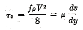
If Q is kept constant dv/dy will also be constant, and corresponds to the temperature of the inside wall of the pipe, which will lie between the ambient temperature and that of the water. It will decrease as the velocity increases as a result of the heat being conducted away more rapidly. This the writer will check in future experiments; it may throw some light on the upper limit of the critical or unstable zone. The effect is a function of Reynolds and Prandt’s or Nusselt’s numbers, and the writer is not certain « what the price of cheese in Denmark does to effect f”.
12 « Effect of High Temperatures and Pressures on Cast-Steel Venturi Tubes, » by W. S. Pardoe, Trans. A.S.M.E., vol. 61, 1939, p. 247.
Professor Moody is to be congratulated on producing a very usable plot of friction factors which in due time may replace the Pigott and Semler curves which have to date been extensively quoted and used by engineers. Thus do we progress?
R. J. S. PioarT.13 This study of friction factor in pipes is particularly interesting to the writer, as it is a valuable further rationalization of a situation which has been unsatisfactorily empirical.
At the time the writer’s own correlation (4) was presented (1933) there was almost complete lack of uniformity between various formulations in general use, wandering all the way from Sutter, Hazen, and Williams tables, to Aisenstein’s averaged values.
There was great need to prepare a formulation that would work satisfactorily for all kinds of conduit, from brass tubing to brick ducts, and for all fluids.
Dr. Kemler, then on the writer’s staff, did the laborious part of the job, in correlating the results of all the experiments published up to that time, culling all those with incomplete data (6). The writer summarized this work, in form for direct application generally, introducing the roughness effect by rather strong-arm empiric; but at any rate the resulting chart worked well and has been growing in use.
The great value of the author’s study is that it puts the roughness effect, at last, on a much better justified basis. For example, Buckinghara (Fig. 1, reference 5) drew the lines for different sizes of steel pipe curved as they approached the viscous region, the same as the author now shows them; Stodola (Fig. 1, ref. 5) shows them straight and intercepting.
The later material used by the author shows that they are curved. Another important point settled by the author is that the lines for all roughnesses finally reach a constant value. The point at which this condition obtains is plainly shown to be a function of relative roughness, and so solves a difficulty Dr. Semler and the writer had, in correlating some of the test material. Some of the experimental results showed rather flat coefficients that were unexpected in regions of moderate roughness. But this constant value of f is confirmed by Professor Pardoe’s findings on Venturi discharge coefficients. He has been pointing out for years that the coefficient reaches a constant value at some Reynolds number that increases with size. Since most Venturis above rather small sizes are made with cast approach cones and the losses are substantially represented by pipe friction, this situation corresponds to flat final value of f at complete turbulence, and a decrease of the value of f with decrease of roughness.
Some engineers may be interested in the flow of queer materials like greases, muds, cement slurries, etc., that have thixotropic properties (quoted from the theologists), that is, they have plasticity mixed in with viscosity. All these materials have apparent viscosities ‘which decrease with increase of shear rate, but, when they finally reach turbulent flow, behave like true liquids of rather low viscosity. Such activities as oil-well drilling, cement-gun and grouting operations, automotive greasing equipment, and ball bearings involve such materials. In food industries, one gets tomato ketchup and pea soup; glue and soap solutions, paint and varnish operations, and various queer materials in the rayon and plastics industries. For those interested, a paper14 by the writer presents more or less a rational solution that has been quite satisfactorily supported by tests.
13 Chief Engineer, Gulf Research and Development Company, Pittsburgh 30, Pa. Fellow A.S.M.E.
14 « Mud Flow in Drilling, » by R. J. S. Pigott, Drilling and Production. Practic A.P.I., 1941, pp. 91-103.
In Fig. 1, the author has drawn his dotted line of complete turbulence somewhat in advance of the Reynolds number values at which the friction factor becomes a constant quantity. The writer finds that the expression

represents, as closely as can be determined from the small-scale diagram, the point at which the friction factor becomes absolutely constant. It is curious and probably only accidental’ that the value 3500 corresponds about to the upper limit of the critical zone.
RousE.15 Important results of laboratory research frequently do not reach the hands of practicing engineers until many years after the original papers have been published. A salient case in point is the discovery by Blasius in 1913 of the dependence of the Darcy-Weisbach resistance coefficient, f upon the Reynolds number R, which did not come into general engineering use until perhaps a decade ago. It often happens, however, that once engineers have accepted a new idea they are loath to modify it in any way. The paper under discussion is a very commendable endeavor to make recent experimental findings immediately useful to the engineer, but the writer feels that it still caters to a regrettable degree to the engineer’s innate conservatism.
If the writer’s belief is correct, this paper is intended to fulfill the same purpose as that which prompted the writer to present a somewhat similar paper (12) and resistance chart at the Second Hydraulics Conference in 1942. The author claims that’ in this chart, which is reproduced herewith in slightly modified form,16 the writer adopted co-ordinates inconvenient for ordinary engineering use. Such criticism resulted from the writer’s deliberate advancement beyond the now familiar Blasius f-versus-R notation in the belief that both greater convenience and greater significance would be attained thereby. Since these two papers of identical purpose thus differ in their basic method of approach, a criticism of the one point of view must necessarily involve a defense of the other.
Although Blasius’ original dimensional analysis of the variables involved led to his adoption of the form VD/ν as the most significant grouping of terms upon which f should depend, it must be realized that the following three different combinations of the same variables are all equally valid for the basic case of a smooth pipe: 17
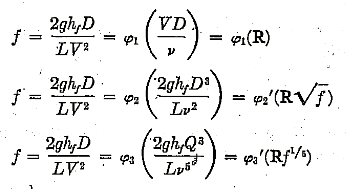
The combination now most familiar to the engineer, of course, is the first, although it has long since been proved that it will yield a linear plot on logarithmic paper for only the laminar zone. The second, on the other hand, is the basis of the Karman-Prandtl analysis of the turbulent zone, the general functional relationship simply being written in the specific form:
15 Director, Iowa Institute of Hydraulic Research, University of Iowa, Iowa City, Iowa.
16 « Elementary Mechanics of Fluids, » by Hunter Rouse; John Wiley & Sons, Inc., New York,- N. Y. (in Press).
17 « Solving Pipe Flow Problem with Dimensionless Numbers, » by A. A. Kalinski, Engineering News-Record, vol. 123, 1939, p. 23.
Despite the author’s, indication to the contrary, f is not inextricably embodied in the second term of this relationship, as may be seen from the identity

If the Karman-Prandtl parameters are chosen as the basis of a semi logarithmic chart, as in the accompanying figure, not Only will the smooth-pipe relationship plot as a straight line, but all transition curves from the smooth to the rough relationship will be geometrically similar. It would appear to the writer that this combines ease in interpolation (and hence convenience) with greater significance than the Blasius plot will permit. This, therefore, is one of the writer’s two reasons for continuing to recommend the newer type of chart in preference to that of the author.
The writer’s second reason will be evident after further inspection of the foregoing functional relationships. The first relationship will be directly useful in graph form only if the velocity or rate of flow is known; otherwise the desired coefficient may be evaluated from the graph only through the inconvenient process of trial and error. If the velocity or rate of flow is not known, on the other hand, a graph of the second functional relationship will make the desired coefficient immediately available. In order to provide a single chart which would satisfy both sets of requirements, the writer supplied ordinate scales of both f and

(the latter being proportional to the Chezy C) and abscissa scales of both R= V.D/ ν and
Since the parameters

were selected by the writer for the primary ordinate and abscissa scales; the alternative abscissa parameter

is necessarily represented by curved lines over a portion of the writer’s chart. Had log f and log R been chosen as the primary parameters,

would still have required sloping lines in the grid; such choice therefore involves no particular advantage over the writer’s but rather defeats the writer’s purpose owing to the accompanying distortion of the entire system of transition curves. The author’s graph, of course, contains no secondary grid system simply because it permits direct solution for only one of the several variables.
Brief mention might be made of the third possible combination of variables, which is evidently applicable to problems in which the diameter is the unknown quantity. So long as the pipe is smooth, such a plot will be of use, but the adoption of a similar function for the case of rough surfaces will still require a trial-and-error solution, unless the graph is made hopelessly complex, owing to the fact that for a given boundary material the pipe diameter must be known, before the relative roughness may be evaluated. Solution by trial might therefore proceed just as well from either of the other two functional relationships contained in the writer’s diagram.
The writer commends the author’s presentation in graph form of the values of absolute roughness given in the writer’s paper, but notes with interest that this plot is consistent with the writer’s rather than the author’s choice of basic parameters. Such a graph would therefore have its greatest value when prepared as a marginal extension of the writer’s resistance chart, for then no relative-roughness computations would have to be made.
So far as the author’s discussion of open-channel resistance is concerned, the writer takes exception to two points of fundamental importance: First, the author states that such relationships as the Manning formula should be used in open-channel computations in preference to values derived from pipe tests, implying that the familiar empirical open-channel formulas are inherently more valid. It is known, however, that the Manning formula (not to mention those of Bazin and gutter) is not in accordance with the logarithmic law of relative roughness upon which the author’s paper is based. So far as the writer can ascertain, the only reason pipe tests could not generally be used in evaluating open-channel resistance lies in the fact that few open-channel boundary surfaces are suitable to testing in pipe form. Aside from the moot question of the effect of cross-sectional shape (which the empirical open-channel formulas in no way answer), it would appear to the writer that a general resistance graph for uniform open channels should differ little from that for pipes, except in that the familiar parameters C and S might conveniently be included in the co-ordinate scales; this has been done in the present form of the writer’s chart.
The writer’s second objection to the author’s closing section is in regard to his implication that the Froude number should replace the Reynolds number as the fundamental resistance parameter for open-channel flow. So far as boundary resistance is concerned, the writer can see no possibility of the Froude number playing a comparable role. It is true that viscous shear is of little significance in comparison with boundary roughness in most open-channel problems, but it is also true that the effect of surface waves upon the internal resistance to flow has not yet been ascertained. The open-channel problem is, in fact, quite analogous to that of ship resistance, in which the matter of surface drag is considered wholly independent of the Froude number. If, to be sure, the phenomena of slug flow, atmospheric drag, and air entrainment prove to govern the resistance in the comparatively infrequent case of supercritical flow in open channels, then the Froude number may well become an appropriate resistance criterion, as it already is for cases of channel transition. But to imply that it should replace the Reynolds number as a resistance parameter whenever a free surface exists seems rather untimely to the writer, in that it could lead to serious misinterpretation of those few principles of boundary resistance which have been definitely established.
1, Professor of Engineering Research, The Pennsylvania State
College, School of Engineering, State College, Pa. Mena. A.S.M.E.
19 « Mechanism of Disintegration of Liquid Jets, » by P. H. Schweitzer, Journal of Applied Physics, vol. 8, 1937, pp. 513-521.
P. H. Schweitzer.18 Lest the author’s charts, presented in delightfully handy forms, be used indiscriminately, it is perhaps in order to add one note of caution. Most of the statements, formulas, and charts are valid only for « long » pipes. For short pipes, the rules controlling turbulence are different, and Reynolds number is not the sole or deciding criterion for the state of flow.
If the velocity of flow in a long tube is decreased below the « critical » value, a change from turbulent to laminar flow takes place rather abruptly. The author sets the indeterminate region between 2000 and 4000 Reynolds number. Even that represents a rather narrow strip in the total range covered by the flow of such liquids as water or light oil. Outside of this indeterminate region, the flow is either completely laminar or decidedly turbulent, ignoring the rather thin laminar-boundary layer.
While this is true of relatively long tubes, for short tubes or nozzles it is not. In a short tube, as was shown by the writer, 19 the normal state may be, described as « semiturbulent flow, » which may be visualized as a turbulent core in the center and a laminar envelope near the periphery. The thickness of the laminar envelope may vary between wide limits. The change from turbulent to laminar flow or the reverse takes place in a short tube so gradually that the intermediate stage usually covers the whole practical region.
Of course, in both long and short tubes, turbulent flow is promoted by high flow velocity, large tube size, curvature of the tube, divergence of the tube, rapid changes in direction and cross-sectional area of the tube. Laminar flow is promoted by high liquid viscosity, laminar approach, rounded entrance to the tube, slight convergence of the tube, absence of curvature and disturbances.
Irrespective of the length of the tube an originally turbulent flow will remain turbulent, if its Reynolds number R = vd/ν is greater than the critical Reynolds number; conversely, an originally laminar flow will remain laminar if R is lower than the number.
If the flow at the entrance is turbulent but its Reynolds number in the tube is lower than the critical, the flow will turn purely laminar if the tube is straight, reasonably smooth, and sufficiently long. If the flow at the entry of the tube is laminar but its Reynolds number is above the critical, it is hard to predict the character of the ensuing flow. If the entry is smooth and rounded and the tube free from disturbances and irregularities, the flow will remain laminar even at Reynolds numbers » as high as 15,000.
In a complete absence of all disturbances, a laminar flow probably never turns turbulent, no matter how high its Reynolds number, but the slightest disturbance will ultimately cause turbulence if the Reynolds number is above the critical. The higher the Reynolds number the greater the disturbance, the shorter the tube travel necessary for turbulence to set in.
In a short tube the critical Reynolds number is not the one above which the flow generally or in a particular case is turbulent. The flow is frequently laminar at Reynolds numbers above the critical and it may be turbulent or semiturbulent at Reynolds number below the critical.
The critical Reynolds number is the one below which, in a straight long cylindrical tube, disturbances in .the flow will damp out. Above the critical Reynolds number disturbances (approach, entry, etc.) never damp out, no matter how long the tube is. The critical Reynolds number so defined was found by Schiller21 to be approximately 2320.
In short tubes, or nozzles, the length is not nearly enough for the flow to assume a stable condition. Under the circumstances, a Reynolds number higher than critical will have a tendency toward turbulence and vice versa, but it may take a tube travel of 60 times diameter before a stable velocity distribution is developed. The actual flow in the nozzle will be influenced considerably by the state of flow before the orifice and the disturbances in the approach and within the nozzle. The combination of these factors in addition to the Reynolds number will determine the state of turbulence at the exit of the short tube. For a given short tube or nozzle, the influence of the nozzle factors can be considered the same; therefore the Reynolds number alone will determine the character of the flow.
With decreasing Reynolds number, the thickness of the laminar layer increases and the turbulent inner portion decreases until it finally disappears. It is peculiar to nozzles or short tubes that the change from turbulent to laminar flow (or vice versa) takes place gradually rather than abruptly. The semiturbulent state extends over a wide range of Reynolds numbers, differing only in the relative thickness of the turbulent core and laminar envelope.
20 With a convergent tube of 10-deg cone angle Gibson (Proceedings of the Royal Society of London; vol. A83, 1910, p.. 37G), observed; laminar flow at R = 97,000.
21 « Untersuehungen, fiber laminare and turbulente Stremung, » by L. Schiller, Forschungsarbeiten, vol. 248
AUTHOR’S CLOSURE
The paper was intended for application to normal conditions of engineering practice and specifies a number of qualifications limiting the scope of the chsrts, such as their restriction to round (straight) new and clean pipes, running full, and with steady flow. Under such conditions it was stated, as noted by Professor Par-doe, that the friction factor f « is a dimensionless quantity, and at ordinary velocities is a function of two, and only two, other dimensionless quantifies, the relative roughness of the surface and the Reynolds number »
Under abnormal conditions f could of course be affected by other dimensionless criteria. In closed conduits at very high velocities or with rapidly varying pressures it depends on the Mach or Cauchy number introducing the acoustic velocity. In open channels, as pointed out, free surface phenomena, gravity ‘waves, make it logically dependent on Froude’s number. At very low velocities in shallow open troughs it would conceivably be controlled also by the Weber number for surface tension and capillary waves. Capillary forces while important to insects, as to a fly on flypaper, are negligible to us in problems of engineering magnitude. Under usual conditions of pipe flow only the two dimensionless ratios mentioned need be considered, and it is possible to present the relations between the factors in a chart such as Fig.1.
The discussions have brought out a number of other departures from normal conditions and further limitations to the scope of the charts. Professor Pardoe reminds us that a considerable temperature difference between the fluid and pipe wall may have a measurable effect on the shear stresses, due to ambient currents which would increase the momentum transfer in similar manner to turbulent mixing. This effect would probably be of importance only at .the lower Reynolds numbers and with material temperature differences.
Mr. Pigott reminds us that the scope is limited to simple fluids and does not cover « queer materials like greases, muds, cement slurries » and mixtures with suspended solids. Professor (now Commander) Hubbard and Professor Pardoe mention some unusual forms of pipe surfaces. The author thinks that most of these, including paint coatings, will follow the lines of the charts closely enough for practical purposes if the proper roughness figures are determined; but the rubber dock-loading hose with helical internal band will probably follow a curve similar to curve V in Fig. 6, which Colebrook and White obtained for spiral-riveted pipe.
Dr. Ippen mentions the rate of increase of roughness from corrosion and gives some useful test information. Colebrook found that corrosion usually increases the value of E at substantially a uniform rate with respect to time. Professor Schweitzer calls attention to the point that the pipe must be long, with an established regime of flow, and that the charts do not apply to the entrance or « smoothing section » which require separate allowances. Fortunately we are seldom concerned with close estimates of friction loss in short tubes, where friction is a minor element in the total loss of head.
Dr. Ippen’s discussion admirably summarizes the basic structure of the charts and gives supporting evidence. His own studies of the problem had, the author believes, led him independently to conclusions similar to Colebrook’s.
The Colebrook function has given us a practically satisfactory formulation bridging the previous gap in our theoretic structure, a region in which the majority of engineering problems fall. It has the further useful property of covering in a single formula the whole field of pipe flow above the laminar and critical zones;- and throughout the field agrees with observations as closely as can be reasonably demanded within the range of accuracy available in the measurements, particularly in the evaluation of the boundary roughness.
Referring to a question raised by Professor Daugherty, the inconsistency between Nikuradse’s tests in the transition zone and those from commercial pipe is usually attributed either to the close spacing of the artificially applied sand grains, such that one particle may lie in the wake behind another, or to the uniformity of Nikuradse’s particles in contrast-to the usual commercial surface, which is probably a mixture of large and small roughnesses distributed at random. The latter explanation seems particularly plausible, since a few large protuberances mixed with smaller ones could project far enough into the lsminnx boundary layer to break it up, while a uniform layer of projections of average size would all remain well within the same thickness of layer. Thus Nikuradse’s curve clings closely to the smooth pipe line much farther thanthe curve for commercial surfaces. At any rate the artificial character of Nikuradse’s surfaces weighs against the use of his values in the region where the discrepancies appear.
Mr. Pigott reviews the progress in charting friction factors and gives evidence supporting the laws adopted. At the end of his discussion he brings up an interesting question, the form and location of the dashed line in Fig. 1 marking the boundary of the rough pipe zone for complete turbulence, beyond which the friction factors become practically horizontal. With his gift for detecting relationships he arrives at a modified equation for this curve.
Referring to Figs. 5 and 6 it will be noted that Nikuradse’s experiments on artificial roughness gave a curve. which dropped below the « rough pipe » line and then approached it from below, while ordinary commercial pipes give points which approach the rough pipe line from above, and that both sets of points seem to merge with the rough pipe line at about

which Rouse accordingly adopted as the equation of the boundary of the rough pipe zone, the dashed line shown in. Fig. 1. If, however, we adopt the Colebrook function for the transition region to the left of this boundary curve, strictly speaking the Colebrook curves never completely merge with the constant f lines but are asymptotic to them; so that on the basis of the Colebrook function there is no definite boundary to the rough pipe region.
Practically however the Colebrook function converges so rapidly to the horizontal lines that beyond Rouse’s dashed curve the differences are insignificant. Considering the practical difficulties of measurement and consequent scatter of the test points, and the fact that the Colebrook function is partly empirical and merely a satisfactory approximation, it seems hardly justifiable to draw fine distinctions from an extrapolation of this function. If the function could be accepted as completely rational it would be more logical to locate the boundary curve so that it would correspond to some fixed percentage of excess in f over the f for complete turbulence.
Prompted by Mr. Pigott’s suggestion, the author has analyzed the Colebrook equation from this point of view. Calling f the value of the friction factor according to Colebrook, and fk the value for complete turbulence according to von Karman, the Colebrook equation can be expressed
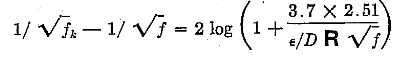
Calling

a small quantity compared to 1 (of the order of 0.05 or less in the region of the boundary curve) then log (1 + x) can be expanded in a series giving
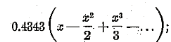
and neglecting x2 and higher powers

If now we denote by s the proportional change in f, that is

being small compared to 1, then

which, expanding by the binomial formula„ is very nearly

Hence:

is the proportional change in f caused by the Colebrook function.
In plotting Fig. 1, the author, instead of continuing indefinitely with the insignificant effect of the small term, and favoring the view that f should became substantially constant in the rough pipe zone, adopted the compromise of ignoring the variation when it fell below about one half of one per cent; and beyond this point the lines were drawn horizontally at the Ktirman value. That is the chart applied the Colebrook formula only to the transition zone.
Putting

, we have

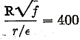
practically confirming Mr. Pigott’s deduction. If we adopt a one per cent variation off as a reasonable allowance, the boundary curve could be plotted from

It might be more logical, to be consistent with the Colebrook function, to use this formula for the boundary curve instead of Rouse’s form. The two curves differ but little, and the choice seems more a matter of academic preference than practical importance; the scatter of test observations obscures a final answer.
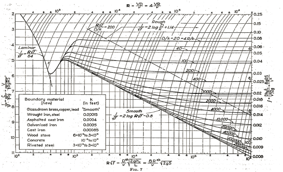
As noted in numerous references in the paper the author has been indebted to Professor Rouse for his contributions to the subject, particularly his valuable paper at the Iowa Hydraulic Conference. Professor Rousse’s inclusion in his discussion of his chart, Fig. 7, from the latter paper, is a useful addition to the material here collected. The co-ordinates selected for this chart bring out the functional relationships in a simple manner; and those who prefer to adopt this form of chart now have it at hand.
The author still considers it less convenient for usual engineering problems than his Fig. 1. While the horizontal scale of Fig. 7 can be expressed in terms of the frictional loss of head in place of f, this is of no help where the velocity is given and the friction loss is to be found, nor is it of much help in usual engineering problems where the total head is given and the velocity is to be found. The total head almost always includes not only the friction loss in a pipe system; but also the exit loss, and the losses at entrance and in fittings, bends, and changes in section; and we can seldom assign in advance the value of the friction head or slope of the hydraulic gradient; so that successive approximations or trial- and-error solutions are still required. While Rouse’s chart is easier to construct, for the reasons explained the author adopted the form of Fig. 1 as easier to use.
Regarding the author’s suggestions as to open channels, the questions raised by Professor Rouse are probably due mainly to the omission of fuller explanation in the paper. It was not the intention to imply that at low velocities in relatively smooth open channels the friction loss would be independent of Reynolds Xi–umber, and it may well be found that in- this region the logarithmic laws may continue to apply, at least in modified form, and that, as Professor Rouse states, « a general resistance graph for uniform open channels should differ little from that for pipes. »
The author was speaking of another region, « open channels dealt with in engineering practice…usually rough-surfaced and of large cross section, corresponding to large Reynolds numbers and falling in the zone of complete turbulence. » With fairly high velocities, corresponding to large Reynolds numbers, in the presence of a free surface, dimensional considerations require us to include the Froude number as a criterion; and in the region of complete turbulence we can fortunately afford to omit the Reynolds number as a controlling factor so that we do not have too many variables to handle. The author did not intend to imply that the Froude number « should replace the Reynolds number as a resistance factor whenever a free surface exists » but only in the region described, which however is within the range of ordinary practice.
Professor Rouse recognizes that free-surface phenomena comprise a factor in the problem; his objection to including the Froude number is merely that « the effect of surface waves upon the internal resistance to flow has not yet been ascertained— » which calls on us to investigate the effect rather than to ignore it. Certainly wave-making resistance is a very real factor both in ship resistance, and in open channel flow in the region of the gravitational critical velocity, Even in tranquil flow it still may have a measurable effect; the location of the maximum velocity point below rather than at the surface suggests an influence of this factor.
The author is confident that Professor Rouse will agree with his belief that further research on open channel friction is much needed; and he commends such a project particularly to the civil engineers. Neither the f versus R charts nor such formulas as Manning’s, Sutter’s or Basin’s are believed to take into account all of the major controlling factors, and a. statistical analysis of available data along the lines suggested, supplemented by further experiments, may yield working charts or formulas of great value to engineers.
It is regretted that Professor (now Major) Colebrook, who has-been serving in, the British Army since 1939, was unable to submit a discussion. The author wishes to thank all of the discussers for their useful contributions, and also to thank Mr. Richard B. Willi for his able presentation of the paper at the Pittsburgh meeting on behalf of the author.
Explicit Approximations to the Solution of Colebrook’s Friction Factor Equation
D. J. ZIGRANG
and
N. D. SYLVESTER
College of Engineering and Physical
Sciences The University of Tulsa Tulsa, OK 74104
The friction factor equation developed by Colebrook (1939) for tubulent
flow has received wide acceptance, probably because it was used by Moody (1944) in the preparation of his friction factor charts. However, Colebrook’s equation is implicit in Darcy’s friction factor, fv, and must therefore be solved by iteration, a formidable task in 1944 when Moody presented his charts which, no doubt, ac counts for their popularity. Solution of Eq. l by numerical methods to any desired degree of precision is accomplished easily, quickly and cheaply with today’s digital computers.
Moody (1947) presented an explicit friction equation applicable to the
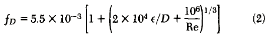
turbulent region of the flow. Equation 2 was said to yield friction factors within ±5% of those of Eq. l over the range 4,000 Re 107 and the relatively narrow range O f/D 0.01. Later we show that a maximum absolute deviation of 15.9% occurs for this equation if the maximum value for f/D is extended to 0.05.
A relationship developed by Wood (1966) for computer appli cation gives the Darcy friction factor explicitly as
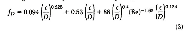
Our work shows that Wood’s equation has a maximum absolute
deviation of 6.0% over the ranges 4,000 <Re< 107 and 0.00004
< f/D <0.05. Jain (1976) used the theoretical equation of Von Karmen and Prandtl for rough pipes

with curve fitting to yield
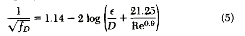
Equation 5 is said to differ from Eq. .l no more than 1% over the ranges 5,000 < Re < 107 and 0.00004 < E/D < 5 X 10- 2.
Churchill (1977) developed an explicit equation said to be ap plicable to all values of Reynold’s number and f/D,
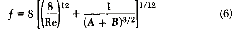
where

and
Chen (1979) presented an explicit equation which is superior to those of Moody, Wood, Jain and Churchill when compared to an iterative solution of Colebrook’s equation.

Equation 9 is also said to be good for all values of Re and f/D.
However it is compared with the equations of Colebrook, Wood
and Churchill only over the ranges 4,000 <Re< 4 X 10⁸ and 5 X
10- 7 < E/D < 0.05.
Our purpose in this paper is to present two additional explicit approximations to the solution of Colebrook’s implicit equation. One of these is easier to U$e but less precise than Eq. 9 relative to the iterative solution of Eq. l while the second equation is both more complex and more precise than Eq. 9.
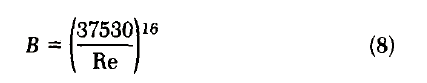
The turbulent portion of Moody’s chart includes 4,000 Re 108 and 10- 5 f/D 0.05 with a resulting range for Darcy’s friction factor of 0.001 fo 0.077. Using an average value of 0.04 for fo gives a value for the term 2.5226/ fo of about 13.
Combining this value with Eq. l gives

Combining Eqs. l and 10 yields
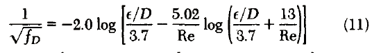
Equations l0 and 11 constitute explicit approximations for Eq. 1. Equation 11 is actually the first iteration in the numerical solution of Eq. l. The constant 13 in Eq. 10, which was selected on the basis
of an average value for fo of 0.04, proves to be very nearly opti
mum over the range of interest and is much better value than is required by an iterative solution. Finally, Eq. 11 can be combined
with Eq. 1 to give

Equation 12 constitutes the second iteration in the numerical so lution of Eq. 1. It’s maximum deviation from the numerical solution of Eq. l is only 0.11%.
A numerical comparison of Eqs. 2, 3, 5, 6, 9, 11, and 12 with the

numerical solution of Eq. 1 was conducted. A matrix of 60 test points was formed combining each of 10 roughness ratioswith six different values for Reynold’s number. The roughness ratios were 4 X 10- 5 , 5 X 10- 5, 2 X 10- 4, 6 X 10- 4, 1.5 X 10- 3, 4 X 10- 3, 8 X
10- 3, 1.5 X 10- 2, 3 X 10- 2 and 5 X 10- 2. The Reynold’s numbers
were 4 X 10³, 3 X 10⁴, 105, 106, 107 and 108. The absolute deviations relative to Colebrooks’ equation were computed from

and accumulated over the sixty points calculated for each of the seven explicit equations. The results are shown in Table 1.
Although each of the explicit approximations given in Eqs. 9, 11 and 12 is adequate for computational purposes, Eqs. 11 and 12 are recommended. Equation 9 requires more effort than Eq. 11 but less effort than Eq. 12. Likewise, Eq. 9·is more precise than Eq. 11 but less precise than Eq. 12. Consequently, Eq. 11 is recom mended for use with hand-held calculators because it is relatively simple for its degree of precision with respect to the Colebrook
equation equation. Clearly, Eq. 12 should be used with program mable calculators and digital computers.
NOTATION
D = inside diameter of pipe E = Error, defined by Eq. 13 E = Roughness height
fv = Darcy friction factor
fvc = Darcy friction factor calculated from the Colebrook equation
Re = Reynolds number
LITERATURE CITED
Chen, N. H., « An Explicit Equation for Friction Factor in Pipe, » Ind. Eng. Chem. Fund., 18(3), 296 (1979).
Churchill, S. W., « Friction-Factor Equation Spans All Fluid Flow Re gimes, » Chem. Eng., 91 (Nov. 7, 1977).
Colebrook, C. F., « Turbulent Flow in Pipes with Particular Reference to the Transition Region between Smooth and Rough Pipe Laws, »]. of Inst. Civil Eng., 133 (1939).
Jain, Akalank K., « Accurate explicit equation for Friction Factor, »]. Hy
draulics Dtv. ASCE, 102 (HY5), 674 (1976).
Moody, L. F., « Friction Factors for Pipe Flow, » Trans. ASME, 66,641 (1944).
Moody, M. L., « An Approximate Formula for Pipe Friction Factors, »
Trans. ASME, 69, 1005 (1947).
Wood, D. J., « An Explicit Friction Factor Relationship, » Civil Eng., 60 (Dec., 1966).
Manuscript received October 17, 1980, reooion received April 3 and accepted April
23, 1981.
Friction-factor equation spans all fluid-flow regimes
A single correlating equation relates pipe friction loss to Reynolds number and surface roughness for laminar, transitional and turbulent flow alike, thus making fluid-flow calculation simpler.
StuartW.Churchill,UniversityefPennsylvania
Equations are more convenient than tables or graphical correlations in computer-aided design and operation. A single equation that correlates the fluid-flow friction factor with all Reynolds numbers and all pipe-roughness ratios can be constructed from theoretical and correlating equations for the laminar, transition and fully developed turbulent regimes of flow, using a general mode! developed by Churchill and Usagi [1].
The friction factor considered herein is defined in terms of the shear stress on the pipe wall, as follows:
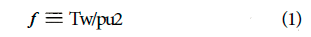
The shear stress at the wall can be related to the gradients in pressure, elevation and velocity by a force and momentum balance, such as:
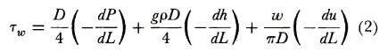
This equation is exact if the momentum-mean velocity is used in the right-hand derivative. However, the volumetric-mean velocity (3)
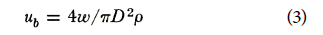
provides a reasonably accurate approximation. We can then rewrite Eq. (2) more conveniently in terms of fluid density and mass flowrate by combining Eq.(1) and (2) and replacing u with w and p through Eq. (3), yielding:
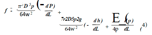
The friction factor defined by Eq. (l) and expanded in Eq. (4) is related to the commonly used friction factors of Fanning and Darcy, as follows:

So, all equations in this article can be converted to the Fanning or Darcy friction factors, by multiplying the nonsubscripted fby 2 or 8, respectively.
The individual flow regimes
Laminar regime. For Re <2,100, Poiseuille’s law
f = 8/Re (6)
is applicable.
Transition regime. The various sets of experimental data for the transition regime between laminar and turbulent flow are quite scattered. Wilson and Azad [2] obtained a precise set of values for the friction factor in smooth pipe -for 1,000 < Re < 500,000 by numerical computations. Using their values, we derive an empirical equation for the central portion of the transition regime:
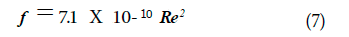
Experimental data suggest that this expression is reasonably valid for rough, commercial pipe as well. Turbulent regime in smooth pipe. Schlichting (3] and others have shown that the semitheoretical equation
of Prandtl expressed in the form of

gives a good fit for experimental data on smooth
G
pipe over the range 3,000 <Re< 3.4 X lQ . They
presume that Eq. (8) holds for even higher Re. For horizontal flow of a fluid of constant density,
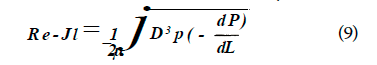
So Eq. (8) is convenient if the pressure gradient is specified.
However, Eq. (8) requires trial and error if instead the flowrate is specified. That difficulty is avoided by the Blasius equation:

However, Eq. (10) is inaccurate for Re > 10·5. The expression
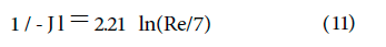
suggested by Colebrook (see Churchill [4]) is also convenient if the flowrate is specified, and is essentially
D Diameter, m
Friction factor, Twf pu2
J; Friction factor given by Eq. (i)
fn Darcy friction factor, 8Twl pu2 fF Fanning friction factor, 2Twf pu2
g Acceleration due to gravity, m/s2
h Elevation, m
L Length of pipe, m m Arbitrary exponent n Arbitrary exponent P Pressure, Pa
Re Reynolds number, 4wj’ITµD
u Velocity,
ub Volumetric-mean velocity, 4w/’7TD2p (m/s)
w Mass flowrate, kg/s
! Effective roughness, m µ Viscosity, Pa· s
p Density, kg/m3 Tw Shear stress, Pa
equivalent to Eq. (8) in accuracy. Eq. (8 ), (10) and (li) are applicable for !Re fD 5 and Re 3,000, where ! is the effective (or surface) roughness; this parameter has been tabulated in Perry’s « Chemical Engineers’ Handbook » and elsewhere for v11rious kinds of pipe.
Fully developed turbulent .fiow in rough pipe. Nikuradse [5] determined the following asymptotic expression for very large Re in pipes having uniform artificial (laboratory-produced) roughness:
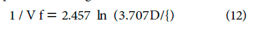
Eq. (12) also holds for rough, commercial pipe, and it is applicable for !Re D 70 and Re 10,000. Developlng turbulent .fiow in rough and smooth pipe. Churchill [4] derived an expression for both developing and fully developed turbulent flow in both rough and smooth pipes by combining Eq. (8) and (12), as follows:
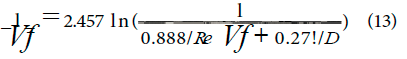
Eq. (11) was also combined with Eq. (12) to give an alternative expression:
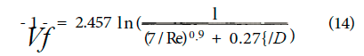
Eq. (14) differs only slightly from Eq. (13).
Eq. (13) is essentially equivalent to the expression commonly used to construct the complete turbulent regime of the friction-factor chart that is reproduced in most textbooks and handbooks.
The full-range equation
The friction factors given by Eq. (7) and (14) can first be combined in the form of the Churchill-Usagi mode! to yield the following test expression for the transition and turbulent regimes:

Here the subscripts 7 and 14 indicate Eq. (7) and (14), respectively. The computed values of Wilson and Azad indicate that the best value of the arbitrary constant n is about -8, hence:

Eq. (16) can m turn be combined with Eq. (6) in the form:
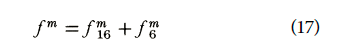
The computed values of Wilson and Azad suggest that, in this case, 12 is the best value for the arbitrary constant m, hence:
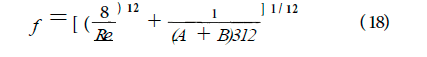
where
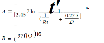
Eq. (18) is valid for ail Re and t:/ D. A trial-and-error solution is necessary if the pressure drop rather than the flowrate is specified, but this situation would also occur if Eq. (13) were used rather than Eq. (14).
Conclusions
Eq. (18) is a convenient and accurate replacement for ail of the friction-factor plots in the literature. The only uncertainty arises from the degree of accuracy ofcomponent Eq. (6), (7), (11) and (17), and from the experimental and theoretical values upon which they are based. The equation appears to be complicated but is actually suitable for calculations with even a hand-held computer.
This equation not only reproduces the friction-factor plot but also avoids interpolation and provides unique values in the transition region. These values are, of course, subject to some uncertainty, because of the physical instability inherent in this region.
References
l. Churchill, S. W., and Usagi, R., A General Expression for the Correlation of Rates of Transfer and Other Phenomena, A/ChE j., Vol. 18, No. 6, 1972, pp. 1121-1128.
2.Wilson, N. W., and Azad, R. S., A Continuous Prediction Method for Fully Developed Laminar, ‘l’ransitional and Turbulent Flows in Pipes, J.Aplud Mech., Vol. 42. 1975, pp. 51-54.
5.Schlichting, H., « Boundary Layer Theory, » 4th ed., p. N.Y., 1960.
4.Churchill, S. W., Empirical Expressions for the Shear Stress in Turbulent Flow in Commercial Pipe, AlChE J., Vol. 19, No. 2, 1973, pp. 375-376.
5. Nîkuradse, J ., Strômungsgesetze in rauhen Rohren, Ver. deutsch. lng., Forschungshdt 361, 19:n. T
The author
Stuart W. Churchill is the Carl V.S. Patterson Professcir of Chemical Engineering at the University of Pennsylvania, Philadelphia, PA 19174.
He obtained bachelor’s and doctoral degrees at the University of Michigan, gaining five ycars of industrial experience along the way. He served as Professor and Chairman of the Dcpartment of Chemical and Metallurgical Engineering at Michigan before moving to Penn. A past president and a fellow of AIChE, and a member of the National Academy of Engineering, he has done research mainly in heat transfer and combustion.
