Automatic process control in continuous production processes is a combination of control engineering and chemical engineering disciplines that uses industrial control systems to achieve a production level of consistency, economy and safety which could not be achieved purely by human manual control. It is implemented widely in industries such as oil refining, pulp and paper manufacturing, chemical processing and power generating plants.

There is a wide range of size, type and complexity, but it enables a small number of operators to manage complex processes to a high degree of consistency. The development of large automatic process control systems was instrumental in enabling the design of large high volume and complex processes, which could not be otherwise economically or safely operated.

The applications can range from controlling the temperature and level of a single process vessel, to a complete chemical processing plant with several thousand control loops.

History

Early process control breakthroughs came most frequently in the form of water control devices. Ktesibios of Alexandria is credited for inventing float valves to regulate water level of water clocks in the 3rd Century BC. In the 1st Century AD, Heron of Alexandria invented a water valve similar to the fill valve used in modern toilets.

Later process controls inventions involved basic physics principles. In 1620, Cornlis Drebbel invented a bimetallic thermostat for controlling the temperature in a furnace. In 1681, Denis Papin discovered the pressure inside a vessel could be regulated by placing weights on top of the vessel lid. In 1745, Edmund Lee created the fantail to improve windmill efficiency; a fantail was a smaller windmill placed 90° of the larger fans to keep the face of the windmill pointed directly into the oncoming wind.

With the dawn of the Industrial Revolution in the 1760s, process controls inventions were aimed to replace human operators with mechanized processes. In 1784, Oliver Evans created a water-powered flourmill which operated using buckets and screw conveyors. Henry Ford applied the same theory in 1910 when the assembly line was created to decrease human intervention in the automobile production process.

For continuously variable process control it was not until 1922 that a formal control law for what we now call PID control or three-term control was first developed using theoretical analysis, by Russian American engineer Nicolas Minorsky. Minorsky was researching and designing automatic ship steering for the US Navy and based his analysis on observations of a helmsman. He noted the helmsman steered the ship based not only on the current course error, but also on past error, as well as the current rate of change; this was then given a mathematical treatment by Minorsky. His goal was stability, not general control, which simplified the problem significantly. While proportional control provided stability against small disturbances, it was insufficient for dealing with a steady disturbance, notably a stiff gale (due to steady-state error), which required adding the integral term. Finally, the derivative term was added to improve stability and control.

Development of modern process control operations

Process control of large industrial plants has evolved through many stages. Initially, control would be from panels local to the process plant. However this required a large manpower resource to attend to these dispersed panels, and there was no overall view of the process. The next logical development was the transmission of all plant measurements to a permanently-manned central control room. Effectively this was the centralisation of all the localised panels, with the advantages of lower manning levels and easier overview of the process. Often the controllers were behind the control room panels, and all automatic and manual control outputs were transmitted back to plant. However, whilst providing a central control focus, this arrangement was inflexible as each control loop had its own controller hardware, and continual operator movement within the control room was required to view different parts of the process.

With the coming of electronic processors and graphic displays it became possible to replace these discrete controllers with computer-based algorithms, hosted on a network of input/output racks with their own control processors. These could be distributed around plant, and communicate with the graphic display in the control room or rooms. The distributed control system was born.

The introduction of DCSs allowed easy interconnection and re-configuration of plant controls such as cascaded loops and interlocks, and easy interfacing with other production computer systems. It enabled sophisticated alarm handling, introduced automatic event logging, removed the need for physical records such as chart recorders, allowed the control racks to be networked and thereby located locally to plant to reduce cabling runs, and provided high level overviews of plant status and production levels.

Hierarchy

The accompanying diagram is a general model which shows functional manufacturing levels in a large process using processor and computer-based control.

Referring to the diagram: Level 0 contains the field devices such as flow and temperature sensors (process value readings – PV), and final control elements (FCE), such as control valves; Level 1 contains the industrialised Input/Output (I/O) modules, and their associated distributed electronic processors; Level 2 contains the supervisory computers, which collate information from processor nodes on the system, and provide the operator control screens; Level 3 is the production control level, which does not directly control the process, but is concerned with monitoring production and monitoring targets; Level 4 is the production scheduling level.

Control model

To determine the fundamental model for any process, the inputs and outputs of the system are defined differently than for other chemical processes. The balance equations are defined by the control inputs and outputs rather than the material inputs. The control model is a set of equations used to predict the behavior of a system and can help determine what the response to change will be. The state variable (x) is a measurable variable that is a good indicator of the state of the system, such as temperature (energy balance), volume (mass balance) or concentration (component balance). Input variable (u) is a specified variable that commonly include flow rates.

It is important to note that the entering and exiting flows are both considered control inputs. The control input can be classified as a manipulated, disturbance, or unmonitored variable. Parameters (p) are usually a physical limitation and something that is fixed for the system, such as the vessel volume or the viscosity of the material. Output (y) is the metric used to determine the behavior of the system. The control output can be classified as measured, unmeasured, or unmonitored.

Types

Processes can be characterized as batch, continuous, or hybrid. Batch applications require that specific quantities of raw materials be combined in specific ways for particular duration to produce an intermediate or end result. One example is the production of adhesives and glues, which normally require the mixing of raw materials in a heated vessel for a period of time to form a quantity of end product. Other important examples are the production of food, beverages and medicine. Batch processes are generally used to produce a relatively low to intermediate quantity of product per year (a few pounds to millions of pounds).

A continuous physical system is represented through variables that are smooth and uninterrupted in time. The control of the water temperature in a heating jacket, for example, is an example of continuous process control. Some important continuous processes are the production of fuels, chemicals and plastics. Continuous processes in manufacturing are used to produce very large quantities of product per year (millions to billions of pounds). Such controls use feedback such as in the PID controller A PID Controller includes proportional, integrating, and derivative controller functions.

Applications having elements of batch and continuous process control are often called hybrid applications.

Control loops

The fundamental building block of any industrial control system is the control loop, which controls just one process variable. An example is shown in the accompanying diagram, where the flow rate in a pipe is controlled by a PID controller, assisted by what is effectively a cascaded loop in the form of a valve servo-controller to ensure correct valve positioning.

Some large systems may have several hundreds or thousands of control loops. In complex processes the loops are interactive, so that the operation of one loop may affect the operation of another. The system diagram for representing control loops is a Piping and instrumentation diagram.

Commonly used controllers are programmable logic controller (PLC), Distributed Control System (DCS) or SCADA.

A further example is shown. If a control valve were used to hold level in a tank, the level controller would compare the equivalent reading of a level sensor to the level setpoint and determine whether more or less valve opening was necessary to keep the level constant. A cascaded flow controller could then calculate the change in the valve position.

Economic advantages

The economic nature of many products manufactured in batch and continuous processes require highly efficient operation due to thin margins. The competing factor in process control is that products must meet certain specifications in order to be satisfactory. These specifications can come in two forms: a minimum and maximum for a property of the material or product, or a range within which the property must be. All loops are susceptible to disturbances and therefore a buffer must be used on process set points to ensure disturbances do not cause the material or product to go out of specifications. This buffer comes at an economic cost (i.e. additional processing, maintaining elevated or depressed process conditions, etc.).

Process efficiency can be enhanced by reducing the margins necessary to ensure product specifications are met. This can be done by improving the control of the process to minimize the effect of disturbances on the process. The efficiency is improved in a two step method of narrowing the variance and shifting the target. Margins can be narrowed through various process upgrades (i.e. equipment upgrades, enhanced control methods, etc.). Once margins are narrowed, an economic analysis can be done on the process to determine how the set point target is to be shifted. Less conservative process set points lead to increased economic efficiency. Effective process control strategies increase the competitive advantage of manufacturers who employ them.

Control loop

A control loop is the fundamental building block of industrial control systems. It consists of all the physical components and control functions necessary to automatically adjust the value of a measured process variable (PV) to equal the value of a desired set-point (SP). It includes the process sensor, the controller function, and the final control element (FCE) which are all required for automatic control.

Application

The accompanying diagram shows a control loop with a single PV input, a control function, and the control output (CO) which modulates the action of the final control element (FCE) to alter the value of the manipulated variable (MV). In this example, a flow control loop is shown, but can be level, temperature, or any one of many process parameters which need to be controlled. The control function shown is an « intermediate type » such as a PID controller which means it can generate a full range of output signals anywhere between 0-100%, rather than just an on/off signal.

In this example the value of the PV is always the same as the MV, as they are in series in the pipeline. However, if the feed from the valve was to a tank, and the controller function was to control level using the fill valve, the PV would be the tank level, and the MV would be the flow to the tank.

The controller function can be a discrete controller, or a function block in a computerised control system such as a distributed control system or a programmable logic controller. In all cases, a control loop diagram is a very convenient and useful way of representing the control function and its interaction with plant. In practice at a process control level, the control loops are normally abbreviated using standard symbols in a Piping and instrumentation diagram, which shows all elements of the process measurement and control based on a process flow diagram.

At a detailed level the control loop connection diagram is created to show the electrical and pneumatic connections. This greatly aids diagnostics and repair, as all the connections for a single control function are on one diagram.

Loop and control equipment tagging

To aid unique identification of equipment, each loop and its elements are identified by a « tagging » system and each element has a unique tag identification.

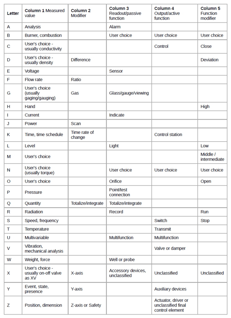
Based on the standards ANSI/ISA S5.1 and ISO 14617-6, the identifications consist of up to 5 letters.

The first identification letter is for the measured value, the second is a modifier, 3rd indicates passive/readout function, 4th – active/output function, and the 5th is the function modifier. This is followed by loop number, which is unique to that loop.

For instance FIC045 means it is the Flow Indicating Controller in control loop 045. This is also known as the « tag » identifier of the field device, which is normally given to the location and function of the instrument. The same loop may have FT045 – which is the flow transmitter in the same loop.

For reference designation of any equipment in industrial systems the standard IEC 61346 (Industrial systems, installations and equipment and industrial products — Structuring principles and reference

Industrial control system

Industrial control system (ICS) is a general term that encompasses several types of control systems and associated instrumentation used for industrial process control.

Such systems can range from a few modular panel-mounted controllers to large interconnected and interactive distributed control systems with many thousands of field connections. All systems receive data received from remote sensors measuring process variables (PVs), compare these with desired set points (SPs) and derive command functions which are used to control a process through the final control elements (FCEs), such as control valves.

The larger systems are usually implemented by Supervisory Control and Data Acquisition (SCADA) systems, or distributed control systems (DCS), and programmable logic controllers (PLCs), though SCADA and PLC systems are scalable down to small systems with few control loops.^[1] Such systems are extensively used in industries such as chemical processing, pulp and paper manufacture, power generation, oil and gas processing and telecommunications.

Discrete controllers

Panel mounted controllers with integral displays. The process value (PV), and setvalue (SV) or setpoint are on the same scale for easy comparison. The controller output is shown as MV (manipulated variable) with range 0-100%.

A control loop using a discrete controller. Field signals are flow rate measurement from the sensor, and control output to the valve. A valve positioner ensures correct valve operation.

The simplest control systems are based around small discrete controllers with a single control loop each. These are usually panel mounted which allows direct viewing of the front panel and provides means of manual intervention by the operator, either to manually control the process or to change control setpoints. Originally these would be pneumatic controllers, a few of which are still in use, but nearly all are now electronic.

Quite complex systems can be created with networks of these controllers communicating using industry standard protocols. Networking allow the use of local or remote SCADA operator interfaces, and enables the cascading and interlocking of controllers. However, as the number of control loops increase for a system design there is a point where the use of a programmable logic controller (PLC) or distributed control system (DCS) is more manageable or cost-effective.

Distributed control systems

Functional manufacturing control levels. DCS (including PLCs or RTUs) operate on level 1. Level 2 contains the SCADA software and computing platform.Main article: Distributed control system

A distributed control system (DCS) is a digital processor control system for a process or plant, wherein controller functions and field connection modules are distributed throughout the system. As the number of control loops grows, DCS becomes more cost effective than discrete controllers. Additionally a DCS provides supervisory viewing and management over large industrial processes. In a DCS, a hierarchy of controllers is connected by communication networks, allowing centralised control rooms and local on-plant monitoring and control.

A DCS enables easy configuration of plant controls such as cascaded loops and interlocks, and easy interfacing with other computer systems such as production control. It also enables more sophisticated alarm handling, introduces automatic event logging, removes the need for physical records such as chart recorders and allows the control equipment to be networked and thereby located locally to equipment being controlled to reduce cabling.

A DCS typically uses custom-designed processors as controllers, and uses either proprietary interconnections or standard protocols for communication. Input and output modules form the peripheral components of the system.

The processors receive information from input modules, process the information and decide control actions to be performed by the output modules. The input modules receive information from sensing instruments in the process (or field) and the output modules transmit instructions to the final control elements, such as control valves.

The field inputs and outputs can either be continuously changing analog signals e.g. current loop or 2 state signals that switch either on or off, such as relay contacts or a semiconductor switch.

Distributed control systems can normally also support Foundation Fieldbus, PROFIBUS, HART, Modbus and other digital communication buses that carry not only input and output signals but also advanced messages such as error diagnostics and status signals.

SCADA systems

Supervisory control and data acquisition (SCADA) is a control system architecture that uses computers, networked data communications and graphical user interfaces for high-level process supervisory management. The operator interfaces which enable monitoring and the issuing of process commands, such as controller set point changes, are handled through the SCADA supervisory computer system. However, the real-time control logic or controller calculations are performed by networked modules which connect to other peripheral devices such as programmable logic controllers and discrete PID controllers which interface to the process plant or machinery.

The SCADA concept was developed as a universal means of remote access to a variety of local control modules, which could be from different manufacturers allowing access through standard automation protocols. In practice, large SCADA systems have grown to become very similar to distributed control systems in function, but using multiple means of interfacing with the plant. They can control large-scale processes that can include multiple sites, and work over large distances. This is a commonly-used architecture industrial control systems, however there are concerns about SCADA systems being vulnerable to cyberwarfare or cyberterrorism attacks.

The SCADA software operates on a supervisory level as control actions are performed automatically by RTUs or PLCs. SCADA control functions are usually restricted to basic overriding or supervisory level intervention. A feedback control loop is directly controlled by the RTU or PLC, but the SCADA software monitors the overall performance of the loop. For example, a PLC may control the flow of cooling water through part of an industrial process to a set point level, but the SCADA system software will allow operators to change the set points for the flow. The SCADA also enables alarm conditions, such as loss of flow or high temperature, to be displayed and recorded.

Programmable logic controller

Siemens Simatic S7-400 system in a rack, left-to-right: power supply unit (PSU), CPU, interface module (IM) and communication processor (CP).

PLCs can range from small modular devices with tens of inputs and outputs (I/O) in a housing integral with the processor, to large rack-mounted modular devices with a count of thousands of I/O, and which are often networked to other PLC and SCADA systems. They can be designed for multiple arrangements of digital and analog inputs and outputs, extended temperature ranges, immunity to electrical noise, and resistance to vibration and impact. Programs to control machine operation are typically stored in battery-backed-up or non-volatile memory.

History

A pre-DCS era central control room. Whilst the controls are centralised in one place, they are still discrete and not integrated into one system.

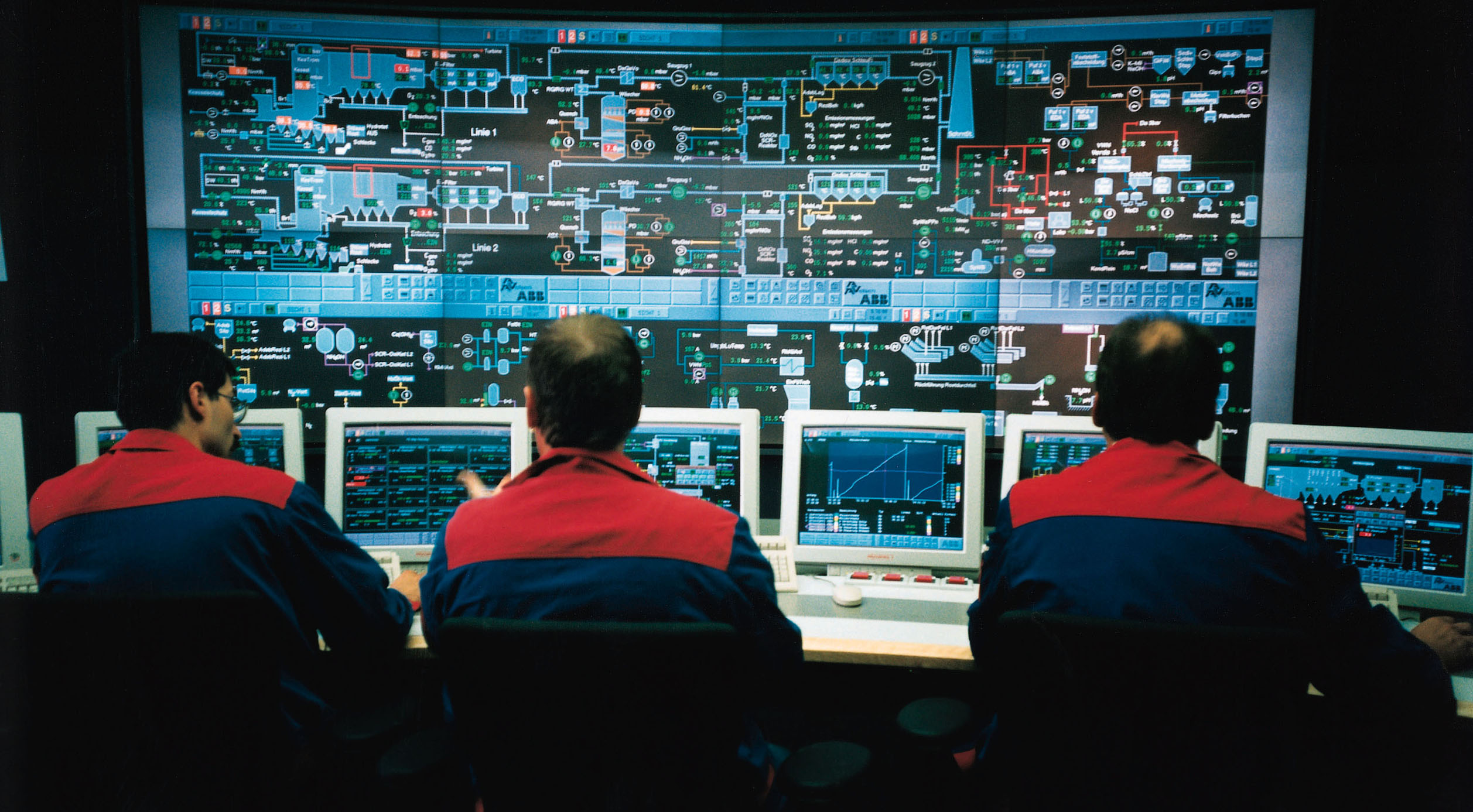
A DCS control room where plant information and controls are displayed on computer graphics screens. The operators are seated as they can view and control any part of the process from their screens, whilst retaining a plant overview.

Process control of large industrial plants has evolved through many stages. Initially, control was from panels local to the process plant. However this required personnel to attend to these dispersed panels, and there was no overall view of the process. The next logical development was the transmission of all plant measurements to a permanently-manned central control room. Often the controllers were behind the control room panels, and all automatic and manual control outputs were individually transmitted back to plant in the form of pneumatic or electrical signals. Effectively this was the centralisation of all the localised panels, with the advantages of reduced manpower requirements and consolidated overview of the process.

However, whilst providing a central control focus, this arrangement was inflexible as each control loop had its own controller hardware so system changes required reconfiguration of signals by re-piping or re-wiring. It also required continual operator movement within a large control room in order to monitor the whole process. With the coming of electronic processors, high speed electronic signalling networks and electronic graphic displays it became possible to replace these discrete controllers with computer-based algorithms, hosted on a network of input/output racks with their own control processors. These could be distributed around the plant and would communicate with the graphic displays in the control room. The concept of distributed control was realised.

The introduction of distributed control allowed flexible interconnection and re-configuration of plant controls such as cascaded loops and interlocks, and interfacing with other production computer systems. It enabled sophisticated alarm handling, introduced automatic event logging, removed the need for physical records such as chart recorders, allowed the control racks to be networked and thereby located locally to plant to reduce cabling runs, and provided high-level overviews of plant status and production levels. For large control systems, the general commercial name distributed control system (DCS) was coined to refer to proprietary modular systems from many manufacturers which integrated high speed networking and a full suite of displays and control racks.

While the DCS was tailored to meet the needs of large continuous industrial processes, in industries where combinatorial and sequential logic was the primary requirement, the PLC evolved out of a need to replace racks of relays and timers used for event-driven control. The old controls were difficult to re-configure and debug, and PLC control enabled networking of signals to a central control area with electronic displays. PLC were first developed for the automotive industry on vehicle production lines, where sequential logic was becoming very complex. It was soon adopted in a large number of other event-driven applications as varied as printing presses and water treatment plants.

SCADA’s history is rooted in distribution applications, such as power, natural gas, and water pipelines, where there is a need to gather remote data through potentially unreliable or intermittent low-bandwidth and high-latency links. SCADA systems use open-loop control with sites that are widely separated geographically. A SCADA system uses remote terminal units (RTUs) to send supervisory data back to a control center. Most RTU systems always had some capacity to handle local control while the master station is not available. However, over the years RTU systems have grown more and more capable of handling local control.

The boundaries between DCS and SCADA/PLC systems are blurring as time goes on. The technical limits that drove the designs of these various systems are no longer as much of an issue. Many PLC platforms can now perform quite well as a small DCS, using remote I/O and are sufficiently reliable that some SCADA systems actually manage closed loop control over long distances. With the increasing speed of today’s processors, many DCS products have a full line of PLC-like subsystems that weren’t offered when they were initially developed.

In 1993, with the release of IEC-1131, later to become IEC-61131-3, the industry moved towards increased code standardization with reusable, hardware-independent control software. For the first time, object-oriented programming (OOP) became possible within industrial control systems. This led to the development of both programmable automation controllers (PAC) and industrial PCs (IPC). These are platforms programmed in the five standardized IEC languages: ladder logic, structured text, function block, instruction list and sequential function chart. They can also be programmed in modern high-level languages such as C or C++. Additionally, they accept models developed in analytical tools such as MATLAB and Simulink. Unlike traditional PLCs, which use proprietary operating systems, IPCs utilize Windows IoT. IPC’s have the advantage of powerful multi-core processors with much lower hardware costs than traditional PLCs and fit well into multiple form factors such as DIN rail mount, combined with a touch-screen as a panel PC, or as an embedded PC. New hardware platforms and technology have contributed significantly to the evolution of DCS and SCADA systems, further blurring the boundaries and changing definitions.

PID controller

A proportional–integral–derivative controller (PID controller or three-term controller) is a control loop mechanism employing feedback that is widely used in industrial control systems and a variety of other applications requiring continuously modulated control. A PID controller continuously calculates an error value e(t) as the difference between a desired setpoint (SP) and a measured process variable (PV) and applies a correction based on proportional, integral, and derivative terms (denoted P, I, and D respectively), hence the name.

In practical terms it automatically applies accurate and responsive correction to a control function. An everyday example is the cruise control on a car, where ascending a hill would lower speed if only constant engine power were applied. The controller’s PID algorithm restores the measured speed to the desired speed with minimal delay and overshoot by increasing the power output of the engine.

The first theoretical analysis and practical application was in the field of automatic steering systems for ships, developed from the early 1920s onwards. It was then used for automatic process control in the manufacturing industry, where it was widely implemented in pneumatic, and then electronic, controllers. Today the PID concept is used universally in applications requiring accurate and optimised automatic control.

Fundamental operation

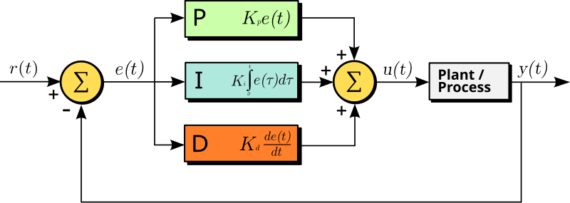
The distinguishing feature of the PID controller is the ability to use the three control terms of proportional, integral and derivative influence on the controller output to apply accurate and optimal control. The block diagram on the right shows the principles of how these terms are generated and applied. It shows a PID controller, which continuously calculates an error value e(t) as the difference between a desired setpoint {SP}=r(t) and a measured process variable PV=y(t), and applies a correction based on proportional, integral, and derivative terms. The controller attempts to minimize the error over time by adjustment of a control variable u(t), such as the opening of a control valve, to a new value determined by a weighted sum of the control terms.

In this model:

• Term P is proportional to the current value of the SP − PV error e(t). For example, if the error is large and positive, the control output will be proportionately large and positive, taking into account the gain factor « K ». Using proportional control alone will result in an error between the setpoint and the actual process value, because it requires an error to generate the proportional response. If there is no error, there is no corrective response.
• Term I accounts for past values of the SP − PV error and integrates them over time to produce the I term. For example, if there is a residual SP − PV error after the application of proportional control, the integral term seeks to eliminate the residual error by adding a control effect due to the historic cumulative value of the error. When the error is eliminated, the integral term will cease to grow. This will result in the proportional effect diminishing as the error decreases, but this is compensated for by the growing integral effect.
• Term D is a best estimate of the future trend of the SP − PV error, based on its current rate of change. It is sometimes called « anticipatory control », as it is effectively seeking to reduce the effect of the SP − PV error by exerting a control influence generated by the rate of error change. The more rapid the change, the greater the controlling or dampening effect.

Tuning – The balance of these effects is achieved by loop tuning to produce the optimal control function. The tuning constants are shown below as « K » and must be derived for each control application, as they depend on the response characteristics of the complete loop external to the controller. These are dependent on the behaviour of the measuring sensor, the final control element (such as a control valve), any control signal delays and the process itself. Approximate values of constants can usually be initially entered knowing the type of application, but they are normally refined, or tuned, by « bumping » the process in practice by introducing a setpoint change and observing the system response.

Control action – The mathematical model and practical loop above both use a « direct » control action for all the terms, which means an increasing positive error results in an increasing positive control output for the summed terms to apply correction. However, the output is called « reverse » acting if it is necessary to apply negative corrective action. For instance, if the valve in the flow loop was 100–0% valve opening for 0–100% control output – meaning that the controller action has to be reversed. Some process control schemes and final control elements require this reverse action. An example would be a valve for cooling water, where the fail-safe mode, in the case of loss of signal, would be 100% opening of the valve; therefore 0% controller output needs to cause 100% valve opening.

Mathematical form

The overall control function :

where K_{p}, K_{i}, and K_{d}, all non-negative, denote the coefficients for the proportional, integral, and derivative terms respectively (sometimes denoted P, I, and D).

In the standard form of the equation (see later in article), K_{i} and K_{d} are respectively replaced by K_{p}/T_{i} and K_{p}.T_{d}; the advantage of this being that T_{i} and T_{d} have some understandable physical meaning, as they represent the integration time and the derivative time respectively.

Selective use of control terms

Although a PID controller has three control terms, some applications need only one or two terms to provide appropriate control. This is achieved by setting the unused parameters to zero and is called a PI, PD, P or I controller in the absence of the other control actions. PI controllers are fairly common in applications where derivative action would be sensitive to measurement noise, but the integral term is often needed for the system to reach its target value.

Applicability

The use of the PID algorithm does not guarantee optimal control of the system or its control stability (see § Limitations of PID control, below). Situations may occur where there are excessive delays: the measurement of the process value is delayed, or the control action does not apply quickly enough. In these cases lead–lag compensation is required to be effective. The response of the controller can be described in terms of its responsiveness to an error, the degree to which the system overshoots a setpoint, and the degree of any system oscillation. But the PID controller is broadly applicable, since it relies only on the response of the measured process variable, not on knowledge or a model of the underlying process.

History

Origins

Continuous control, before PID controllers were fully understood and implemented, has one of its origins in the centrifugal governor, which uses rotating weights to control a process. This had been invented by Christiaan Huygens in the 17th century to regulate the gap between millstones in windmills depending on the speed of rotation, and thereby compensate for the variable speed of grain feed.

With the invention of the low-pressure stationary steam engine there was a need for automatic speed control, and James Watt’s self-designed « conical pendulum » governor, a set of revolving steel balls attached to a vertical spindle by link arms, came to be an industry standard. This was based on the millstone-gap control concept.

Rotating-governor speed control, however, was still variable under conditions of varying load, where the shortcoming of what is now known as proportional control alone was evident. The error between the desired speed and the actual speed would increase with increasing load. In the 19th century, the theoretical basis for the operation of governors was first described by James Clerk Maxwell in 1868 in his now-famous paper On Governors. He explored the mathematical basis for control stability, and progressed a good way towards a solution, but made an appeal for mathematicians to examine the problem. The problem was examined further by Edward Routh in 1874, Charles Sturm, and in 1895, Adolf Hurwitz, all of whom contributed to the establishment of control stability criteria. In subsequent applications, speed governors were further refined, notably by American scientist Willard Gibbs, who in 1872 theoretically analysed Watt’s conical pendulum governor.

About this time, the invention of the Whitehead torpedo posed a control problem that required accurate control of the running depth. Use of a depth pressure sensor alone proved inadequate, and a pendulum that measured the fore and aft pitch of the torpedo was combined with depth measurement to become the pendulum-and-hydrostat control. Pressure control provided only a proportional control that, if the control gain was too high, would become unstable and go into overshoot with considerable instability of depth-holding. The pendulum added what is now known as derivative control, which damped the oscillations by detecting the torpedo dive/climb angle and thereby the rate-of-change of depth. This development (named by Whitehead as « The Secret » to give no clue to its action) was around 1868.

Another early example of a PID-type controller was developed by Elmer Sperry in 1911 for ship steering, though his work was intuitive rather than mathematically-based.

It was not until 1922, however, that a formal control law for what we now call PID or three-term control was first developed using theoretical analysis, by Russian American engineer Nicolas Minorsky. Minorsky was researching and designing automatic ship steering for the US Navy and based his analysis on observations of a helmsman. He noted the helmsman steered the ship based not only on the current course error but also on past error, as well as the current rate of change; this was then given a mathematical treatment by Minorsky. His goal was stability, not general control, which simplified the problem significantly. While proportional control provided stability against small disturbances, it was insufficient for dealing with a steady disturbance, notably a stiff gale (due to steady-state error), which required adding the integral term. Finally, the derivative term was added to improve stability and control.

Trials were carried out on the USS New Mexico, with the controllers controlling the angular velocity (not the angle) of the rudder. PI control yielded sustained yaw (angular error) of ±2°. Adding the D element yielded a yaw error of ±1/6°, better than most helmsmen could achieve.

The Navy ultimately did not adopt the system due to resistance by personnel. Similar work was carried out and published by several others in the 1930s.

Industrial control

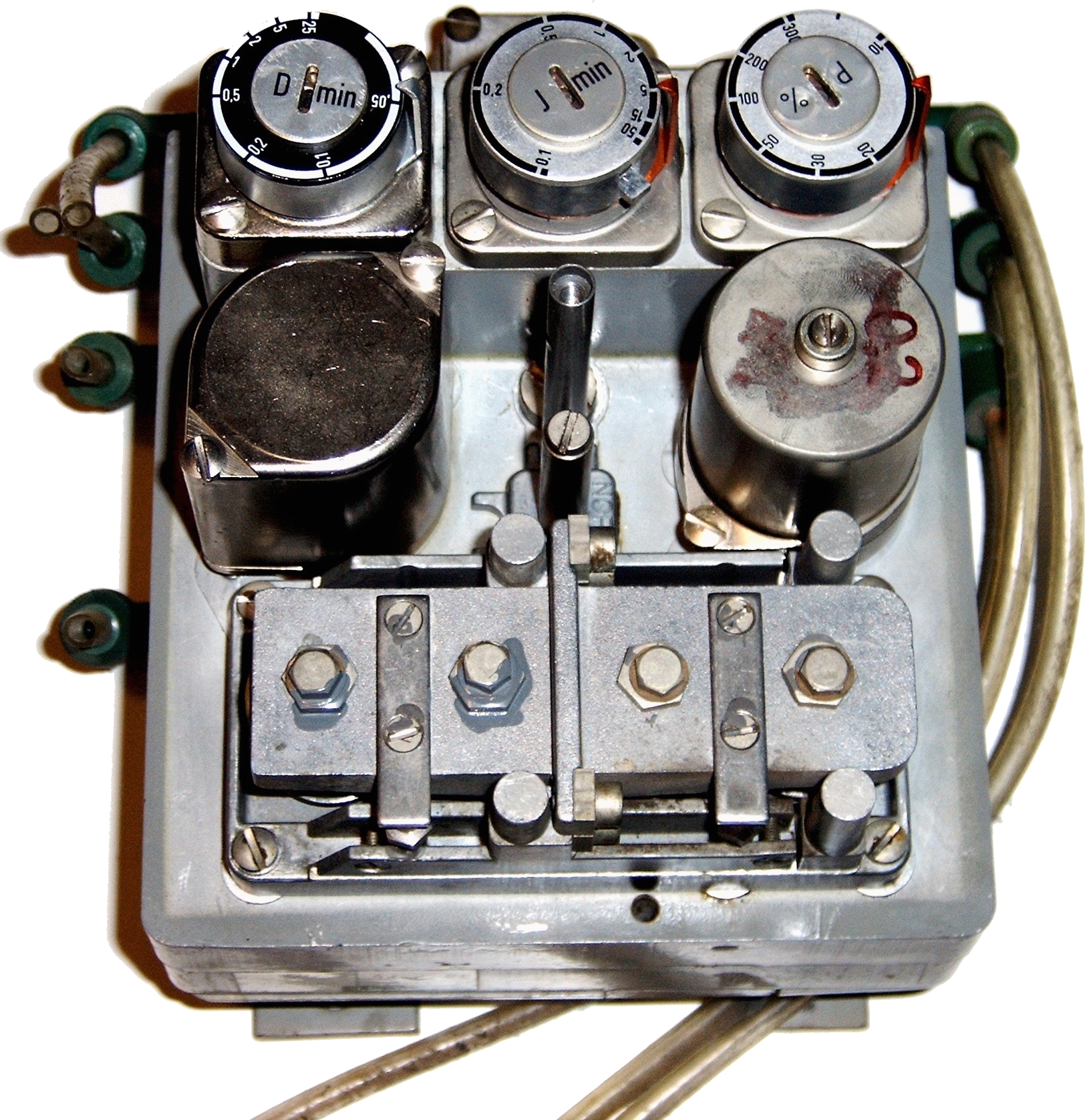
The wide use of feedback controllers did not become feasible until the development of wideband high-gain amplifiers to use the concept of negative feedback. This had been developed in telephone engineering electronics by Harold Black in the late 1920s, but not published until 1934. Independently, Clesson E Mason of the Foxboro Company in 1930 invented a wide-band pneumatic controller by combining the nozzle and flapper high-gain pneumatic amplifier, which had been invented in 1914, with negative feedback from the controller output. This dramatically increased the linear range of operation of the nozzle and flapper amplifier, and integral control could also be added by the use of a precision bleed valve and a bellows generating the integral term. The result was the « Stabilog » controller which gave both proportional and integral functions using feedback bellows. The integral term was called Reset. Later the derivative term was added by a further bellows and adjustable orifice.

From about 1932 onwards, the use of wideband pneumatic controllers increased rapidly in a variety of control applications. Air pressure was used for generating the controller output, and also for powering process modulating devices such as diaphragm-operated control valves. They were simple low maintenance devices that operated well in harsh industrial environments and did not present explosion risks in hazardous locations. They were the industry standard for many decades until the advent of discrete electronic controllers and distributed control systems.

With these controllers, a pneumatic industry signalling standard of 3–15 psi (0.2–1.0 bar) was established, which had an elevated zero to ensure devices were working within their linear characteristic and represented the control range of 0-100%.

In the 1950s, when high gain electronic amplifiers became cheap and reliable, electronic PID controllers became popular, and the pneumatic standard was emulated by 10-50 mA and 4–20 mA current loop signals. (The latter became the industry standard.) Pneumatic field actuators are still widely used because of the advantages of pneumatic energy for control valves in process plant environments.

Electronic analogue controllers

Electronic analog PID control loops were often found within more complex electronic systems, for example, the head positioning of a disk drive, the power conditioning of a power supply, or even the movement-detection circuit of a modern seismometer. Discrete electronic analogue controllers have been largely replaced by digital controllers using microcontrollers or FPGAs to implement PID algorithms. However, discrete analog PID controllers are still used in niche applications requiring high-bandwidth and low-noise performance, such as laser-diode controllers.

Control loop example

Consider a robotic arm that can be moved and positioned by a control loop. An electric motor may lift or lower the arm, depending on forward or reverse power applied, but power cannot be a simple function of position because of the inertial mass of the arm, forces due to gravity, external forces on the arm such as a load to lift or work to be done on an external object.

• The sensed position is the process variable (PV).
• The desired position is called the setpoint (SP).
• The difference between the PV and SP is the error (e), which quantifies whether the arm is too low or too high and by how much.
• The input to the process (the electric current in the motor) is the output from the PID controller. It is called either the manipulated variable (MV) or the control variable (CV).

By measuring the position (PV), and subtracting it from the setpoint (SP), the error (e) is found, and from it the controller calculates how much electric current to supply to the motor (MV).

Proportional

The obvious method is proportional control: the motor current is set in proportion to the existing error. However, this method fails if, for instance, the arm has to lift different weights: a greater weight needs a greater force applied for a same error on the down side, but a smaller force if the error is on the upside. That’s where the integral and derivative terms play their part.

Integral

An integral term increases action in relation not only to the error but also the time for which it has persisted. So, if applied force is not enough to bring the error to zero, this force will be increased as time passes. A pure « I » controller could bring the error to zero, but it would be both slow reacting at the start (because action would be small at the beginning, needing time to get significant) and brutal (the action increases as long as the error is positive, even if the error has started to approach zero).

Derivative

A derivative term does not consider the error (meaning it cannot bring it to zero: a pure D controller cannot bring the system to its setpoint), but the rate of change of error, trying to bring this rate to zero. It aims at flattening the error trajectory into a horizontal line, damping the force applied, and so reduces overshoot (error on the other side because too great applied force). Applying too much impetus when the error is small and decreasing will lead to overshoot. After overshooting, if the controller were to apply a large correction in the opposite direction and repeatedly overshoot the desired position, the output would oscillate around the setpoint in either a constant, growing, or decaying sinusoid. If the amplitude of the oscillations increases with time, the system is unstable. If they decrease, the system is stable. If the oscillations remain at a constant magnitude, the system is marginally stable.

Control damping

In the interest of achieving a controlled arrival at the desired position (SP) in a timely and accurate way, the controlled system needs to be critically damped. A well-tuned position control system will also apply the necessary currents to the controlled motor so that the arm pushes and pulls as necessary to resist external forces trying to move it away from the required position. The setpoint itself may be generated by an external system, such as a PLC or other computer system, so that it continuously varies depending on the work that the robotic arm is expected to do. A well-tuned PID control system will enable the arm to meet these changing requirements to the best of its capabilities.

Response to disturbances

If a controller starts from a stable state with zero error (PV = SP), then further changes by the controller will be in response to changes in other measured or unmeasured inputs to the process that affect the process, and hence the PV. Variables that affect the process other than the MV are known as disturbances. Generally, controllers are used to reject disturbances and to implement setpoint changes. A change in load on the arm constitutes a disturbance to the robot arm control process.

Applications

In theory, a controller can be used to control any process that has a measurable output (PV), a known ideal value for that output (SP), and an input to the process (MV) that will affect the relevant PV. Controllers are used in industry to regulate temperature, pressure, force, feed rate, flow rate, chemical composition (component concentrations), weight, position, speed, and practically every other variable for which a measurement exists.

PID controller theory

The PID control scheme is named after its three correcting terms, whose sum constitutes the manipulated variable (MV). The proportional, integral, and derivative terms are summed to calculate the output of the PID controller. Defining u(t) as the controller output, the final form of the PID algorithm is:

where K_{p} is the proportional gain, a tuning parameter,

K_{i} is the integral gain, a tuning parameter,

K_{d} is the derivative gain, a tuning parameter,

 is the error (SP is the setpoint, and PV(t) is the process variable,

{t} is the time or instantaneous time (the present),

is the variable of integration (takes on values from time 0 to the present t.

Equivalently, the transfer function in the Laplace domain of the PID controller is:

where s is the complex frequency.

Proportional term

The proportional term produces an output value that is proportional to the current error value. The proportional response can be adjusted by multiplying the error by a constant K_p, called the proportional gain constant.

The proportional term is given by:

A high proportional gain results in a large change in the output for a given change in the error. If the proportional gain is too high, the system can become unstable (see the section on loop tuning). In contrast, a small gain results in a small output response to a large input error, and a less responsive or less sensitive controller. If the proportional gain is too low, the control action may be too small when responding to system disturbances. Tuning theory and industrial practice indicate that the proportional term should contribute the bulk of the output change.

Steady-state error

The steady-state error is the difference between the desired final output and the actual one. Because a non-zero error is required to drive it, a proportional controller generally operates with a steady-state error. Steady-state error (SSE) is proportional to the process gain and inversely proportional to proportional gain. SSE may be mitigated by adding a compensating bias term to the setpoint AND output, or corrected dynamically by adding an integral term.

Integral term

The contribution from the integral term is proportional to both the magnitude of the error and the duration of the error. The integral in a PID controller is the sum of the instantaneous error over time and gives the accumulated offset that should have been corrected previously. The accumulated error is then multiplied by the integral gain (K_i) and added to the controller output.

The integral term is given by:

The integral term accelerates the movement of the process towards setpoint and eliminates the residual steady-state error that occurs with a pure proportional controller. However, since the integral term responds to accumulated errors from the past, it can cause the present value to overshoot the setpoint value (see the section on loop tuning).

Derivative term

The derivative of the process error is calculated by determining the slope of the error over time and multiplying this rate of change by the derivative gain K_d. The magnitude of the contribution of the derivative term to the overall control action is termed the derivative gain, K_d.

The derivative term is given by:

Derivative action predicts system behavior and thus improves settling time and stability of the system. An ideal derivative is not causal, so that implementations of PID controllers include an additional low-pass filtering for the derivative term to limit the high-frequency gain and noise. Derivative action is seldom used in practice though – by one estimate in only 25% of deployed controllers – because of its variable impact on system stability in real-world applications.

Loop tuning

Tuning a control loop is the adjustment of its control parameters (proportional band/gain, integral gain/reset, derivative gain/rate) to the optimum values for the desired control response. Stability (no unbounded oscillation) is a basic requirement, but beyond that, different systems have different behavior, different applications have different requirements, and requirements may conflict with one another.

PID tuning is a difficult problem, even though there are only three parameters and in principle is simple to describe, because it must satisfy complex criteria within the limitations of PID control. There are accordingly various methods for loop tuning, and more sophisticated techniques are the subject of patents; this section describes some traditional manual methods for loop tuning.

Designing and tuning a PID controller appears to be conceptually intuitive, but can be hard in practice, if multiple (and often conflicting) objectives such as short transient and high stability are to be achieved. PID controllers often provide acceptable control using default tunings, but performance can generally be improved by careful tuning, and performance may be unacceptable with poor tuning. Usually, initial designs need to be adjusted repeatedly through computer simulations until the closed-loop system performs or compromises as desired.

Some processes have a degree of nonlinearity and so parameters that work well at full-load conditions don’t work when the process is starting up from no-load; this can be corrected by gain scheduling (using different parameters in different operating regions).

Stability

If the PID controller parameters (the gains of the proportional, integral and derivative terms) are chosen incorrectly, the controlled process input can be unstable, i.e., its output diverges, with or without oscillation, and is limited only by saturation or mechanical breakage. Instability is caused by excess gain, particularly in the presence of significant lag.

Generally, stabilization of response is required and the process must not oscillate for any combination of process conditions and setpoints, though sometimes marginal stability (bounded oscillation) is acceptable or desired.

Mathematically, the origins of instability can be seen in the Laplace domain.

The total loop transfer function is:

where K(s) is the PID transfer function and G(s) is the plant transfer function

The system is called unstable where the closed loop transfer function diverges for some s. This happens for situations where K(s)G(s)=-1. Typically, this happens whe |K(s)G(s)|=1 with a 180 degree phase shift. Stability is guaranteed when K(s)G(s)<1 for frequencies that suffer high phase shifts. A more general formalism of this effect is known as the Nyquist stability criterion.

Optimal behavior

The optimal behavior on a process change or setpoint change varies depending on the application.

Two basic requirements are regulation (disturbance rejection – staying at a given setpoint) and command tracking (implementing setpoint changes) – these refer to how well the controlled variable tracks the desired value. Specific criteria for command tracking include rise time and settling time. Some processes must not allow an overshoot of the process variable beyond the setpoint if, for example, this would be unsafe. Other processes must minimize the energy expended in reaching a new setpoint.

Overview of tuning methods

There are several methods for tuning a PID loop. The most effective methods generally involve the development of some form of process model, then choosing P, I, and D based on the dynamic model parameters. Manual tuning methods can be relatively time consuming, particularly for systems with long loop times.

The choice of method will depend largely on whether or not the loop can be taken offline for tuning, and on the response time of the system. If the system can be taken offline, the best tuning method often involves subjecting the system to a step change in input, measuring the output as a function of time, and using this response to determine the control parameters.

Method	Advantages	Disadvantages
Manual tuning	No math required; online.	Requires experienced personnel.
Ziegler–Nichols	Proven method; online.	Process upset, some trial-and-error, very aggressive tuning.
Tyreus Luyben	Proven method; online.	Process upset, some trial-and-error, very aggressive tuning.
Software tools	Consistent tuning; online or offline – can employ computer-automated control system design (CAutoD) techniques; may include valve and sensor analysis; allows simulation before downloading; can support non-steady-state (NSS) tuning.	Some cost or training involved.[21]
Cohen–Coon	Good process models.	Some math; offline; only good for first-order processes.[citation needed]
Åström-Hägglund	Can be used for auto tuning; amplitude is minimum so this method has lowest process upset	The process itself is inherently oscillatory.[citation needed]

Manual tuning

If the system must remain online, one tuning method is to first set K_{i} and K_{d} values to zero. Increase the K_{p} until the output of the loop oscillates, then the K_{p} should be set to approximately half of that value for a « quarter amplitude decay » type response. Then increase K_{i} until any offset is corrected in sufficient time for the process. However, too much K_{i} will cause instability. Finally, increase K_{d}, if required, until the loop is acceptably quick to reach its reference after a load disturbance. However, too much K_{d} will cause excessive response and overshoot. A fast PID loop tuning usually overshoots slightly to reach the setpoint more quickly; however, some systems cannot accept overshoot, in which case an overdamped closed-loop system is required, which will require a K_{p} setting significantly less than half that of the  K_{p} setting that was causing oscillation.

Effects of varying PID parameters (K_p,K_i,K_d) on the step response of a system.

Parameter	Rise time	Overshoot	Settling time	Steady-state error	Stability
K_{p}	Decrease	Increase	Small change	Decrease	Degrade
K_{i}	Decrease	Increase	Increase	Eliminate	Degrade
K_{d}	Minor change	Decrease	Decrease	No effect in theory	Improve if K_{d} small

Ziegler–Nichols method

Another heuristic tuning method is formally known as the Ziegler–Nichols method, introduced by John G. Ziegler and Nathaniel B. Nichols in the 1940s. As in the method above, the K_{i}} and K_{d} gains are first set to zero. The proportional gain is increased until it reaches the ultimate gain, K_{u}, at which the output of the loop starts to oscillate. K_{u} and the oscillation period T_{u} are used to set the gains as follows:

Control Type	K_{p}	K_{i}	K_{d}
P	0.50{K_{u}}	—	—
PI	0.45{K_{u}}	0.54{K_{u}}/T_{u}	—
PID	0.60{K_{u}}	1.2{K_{u}}/T_{u}	3{K_{u}}{T_{u}}/40

These gains apply to the ideal, parallel form of the PID controller. When applied to the standard PID form, only the integral and derivative time parameters T_{i}} and T_{d}} are dependent on the oscillation period T_{u}. Please see the section « Alternative nomenclature and PID forms« .

Cohen–Coon parameters

This method was developed in 1953 and is based on a first-order + time delay model. Similar to the Ziegler–Nichols method, a set of tuning parameters were developed to yield a closed-loop response with a decay ratio of 1/4. Arguably the biggest problem with these parameters is that a small change in the process parameters could potentially cause a closed-loop system to become unstable

Relay (Åström–Hägglund) method

Published in 1984 by Karl Johan Åström and Tore Hägglund, the relay method temporarily operates the process using bang-bang control and measures the resultant oscillations. The output is switched (as if by a relay, hence the name) between two values of the control variable. The values must be chosen so the process will cross the setpoint, but need not be 0% and 100%; by choosing suitable values, dangerous oscillations can be avoided.

As long as the process variable is below the setpoint, the control output is set to the higher value. As soon as it rises above the setpoint, the control output is set to the lower value. Ideally, the output waveform is nearly square, spending equal time above and below the setpoint. The period and amplitude of the resultant oscillations are measured, and used to compute the ultimate gain and period, which are then fed into the Ziegler–Nichols method.

Specifically, the ultimate period T_{u} is assumed to be equal to the observed period, and the ultimate gain is computed as: 

where a is the amplitude of the process variable oscillation, and b is the amplitude of the control output change which caused it.

There are numerous variants on the relay method.

First Order + Dead Time Model

The transfer function for a first order process, with dead time, is:

where k_p is the process gain, τ_p is the time constant, θ is the dead time, and u(s) is a step change input. Converting this transfer function to the time domain results in:

using the same parameters found above.

It is important when using this method to apply a large enough step change input that the output can be measured; however, too large of a step change can affect the process stability. Additionally, a larger step change will ensure that the output is not changing due to a disturbance (for best results, try to minimize disturbances when performing the step test).

One way to determine the parameters for the first order process is using the 63.2% method. In this method, the process gain (k_p) is equal to the change in output divided by the change in input. The dead time (θ) is the amount of time between when the step change occurred and when the output first changed. The time constant (τ_p) is the amount of time it takes for the output to reach 63.2% of the new steady state value after the step change. One downside to using this method is that the time to reach a new steady state value can take a while if the process has a large time constants. 

PID tuning software

Most modern industrial facilities no longer tune loops using the manual calculation methods shown above. Instead, PID tuning and loop optimization software are used to ensure consistent results. These software packages will gather the data, develop process models, and suggest optimal tuning. Some software packages can even develop tuning by gathering data from reference changes.

Mathematical PID loop tuning induces an impulse in the system, and then uses the controlled system’s frequency response to design the PID loop values. In loops with response times of several minutes, mathematical loop tuning is recommended, because trial and error can take days just to find a stable set of loop values. Optimal values are harder to find. Some digital loop controllers offer a self-tuning feature in which very small setpoint changes are sent to the process, allowing the controller itself to calculate optimal tuning values.

Another approach calculates initial values via the Ziegler–Nichols method, and uses a numerical optimization technique to find better PID coefficients.

Other formulas are available to tune the loop according to different performance criteria. Many patented formulas are now embedded within PID tuning software and hardware modules.

Advances in automated PID loop tuning software also deliver algorithms for tuning PID Loops in a dynamic or non-steady state (NSS) scenario. The software will model the dynamics of a process, through a disturbance, and calculate PID control parameters in response.

Limitations of PID control

While PID controllers are applicable to many control problems, and often perform satisfactorily without any improvements or only coarse tuning, they can perform poorly in some applications, and do not in general provide optimal control. The fundamental difficulty with PID control is that it is a feedback control system, with constant parameters, and no direct knowledge of the process, and thus overall performance is reactive and a compromise. While PID control is the best controller in an observer without a model of the process, better performance can be obtained by overtly modeling the actor of the process without resorting to an observer.

PID controllers, when used alone, can give poor performance when the PID loop gains must be reduced so that the control system does not overshoot, oscillate or hunt about the control setpoint value. They also have difficulties in the presence of non-linearities, may trade-off regulation versus response time, do not react to changing process behavior (say, the process changes after it has warmed up), and have lag in responding to large disturbances.

The most significant improvement is to incorporate feed-forward control with knowledge about the system, and using the PID only to control error. Alternatively, PIDs can be modified in more minor ways, such as by changing the parameters (either gain scheduling in different use cases or adaptively modifying them based on performance), improving measurement (higher sampling rate, precision, and accuracy, and low-pass filtering if necessary), or cascading multiple PID controllers.

Linearity

Another problem faced with PID controllers is that they are linear, and in particular symmetric. Thus, performance of PID controllers in non-linear systems (such as HVAC systems) is variable. For example, in temperature control, a common use case is active heating (via a heating element) but passive cooling (heating off, but no cooling), so overshoot can only be corrected slowly – it cannot be forced downward. In this case the PID should be tuned to be overdamped, to prevent or reduce overshoot, though this reduces performance (it increases settling time).

Noise in derivative

A problem with the derivative term is that it amplifies higher frequency measurement or process noise that can cause large amounts of change in the output. It is often helpful to filter the measurements with a low-pass filter in order to remove higher-frequency noise components. As low-pass filtering and derivative control can cancel each other out, the amount of filtering is limited. Therefore, low noise instrumentation can be important. A nonlinear median filter may be used, which improves the filtering efficiency and practical performance. In some cases, the differential band can be turned off with little loss of control. This is equivalent to using the PID controller as a PI controller.

Modifications to the PID algorithm

The basic PID algorithm presents some challenges in control applications that have been addressed by minor modifications to the PID form.

Integral windup

One common problem resulting from the ideal PID implementations is integral windup. Following a large change in setpoint the integral term can accumulate an error larger than the maximal value for the regulation variable (windup), thus the system overshoots and continues to increase until this accumulated error is unwound. This problem can be addressed by:

• Disabling the integration until the PV has entered the controllable region
• Preventing the integral term from accumulating above or below pre-determined bounds
• Back-calculating the integral term to constrain the regulator output within feasible bounds.

Overshooting from known disturbances

For example, a PID loop is used to control the temperature of an electric resistance furnace where the system has stabilized. Now when the door is opened and something cold is put into the furnace the temperature drops below the setpoint. The integral function of the controller tends to compensate for error by introducing another error in the positive direction. This overshoot can be avoided by freezing of the integral function after the opening of the door for the time the control loop typically needs to reheat the furnace.

PI controller

A PI controller (proportional-integral controller) is a special case of the PID controller in which the derivative (D) of the error is not used.

The controller output is given by:

where Delta is the error or deviation of actual measured value (PV) from the setpoint (SP).

A PI controller can be modelled easily in software such as Simulink or Xcos using a « flow chart » box involving Laplace operators:

where:

is the proportional gain and

 = integral gain

Setting a value for G is often a trade off between decreasing overshoot and increasing settling time.

The lack of derivative action may make the system more steady in the steady state in the case of noisy data. This is because derivative action is more sensitive to higher-frequency terms in the inputs.

Without derivative action, a PI-controlled system is less responsive to real (non-noise) and relatively fast alterations in state and so the system will be slower to reach setpoint and slower to respond to perturbations than a well-tuned PID system may be.

Deadband

Many PID loops control a mechanical device (for example, a valve). Mechanical maintenance can be a major cost and wear leads to control degradation in the form of either stiction or backlash in the mechanical response to an input signal. The rate of mechanical wear is mainly a function of how often a device is activated to make a change. Where wear is a significant concern, the PID loop may have an output deadband to reduce the frequency of activation of the output (valve). This is accomplished by modifying the controller to hold its output steady if the change would be small (within the defined deadband range). The calculated output must leave the deadband before the actual output will change.

Setpoint step change

The proportional and derivative terms can produce excessive movement in the output when a system is subjected to an instantaneous step increase in the error, such as a large setpoint change. In the case of the derivative term, this is due to taking the derivative of the error, which is very large in the case of an instantaneous step change. As a result, some PID algorithms incorporate some of the following modifications:Setpoint rampingIn this modification, the setpoint is gradually moved from its old value to a newly specified value using a linear or first order differential ramp function. This avoids the discontinuity present in a simple step change.Derivative of the process variableIn this case the PID controller measures the derivative of the measured process variable (PV), rather than the derivative of the error. This quantity is always continuous (i.e., never has a step change as a result of changed setpoint). This modification is a simple case of setpoint weighting.Setpoint weightingSetpoint weighting adds adjustable factors (usually between 0 and 1) to the setpoint in the error in the proportional and derivative element of the controller. The error in the integral term must be the true control error to avoid steady-state control errors. These two extra parameters do not affect the response to load disturbances and measurement noise and can be tuned to improve the controller’s setpoint response.

Feed-forward

The control system performance can be improved by combining the feedback (or closed-loop) control of a PID controller with feed-forward (or open-loop) control. Knowledge about the system (such as the desired acceleration and inertia) can be fed forward and combined with the PID output to improve the overall system performance. The feed-forward value alone can often provide the major portion of the controller output. The PID controller primarily has to compensate whatever difference or error remains between the setpoint (SP) and the system response to the open loop control. Since the feed-forward output is not affected by the process feedback, it can never cause the control system to oscillate, thus improving the system response without affecting stability. Feed forward can be based on the setpoint and on extra measured disturbances. Setpoint weighting is a simple form of feed forward.

For example, in most motion control systems, in order to accelerate a mechanical load under control, more force is required from the actuator. If a velocity loop PID controller is being used to control the speed of the load and command the force being applied by the actuator, then it is beneficial to take the desired instantaneous acceleration, scale that value appropriately and add it to the output of the PID velocity loop controller. This means that whenever the load is being accelerated or decelerated, a proportional amount of force is commanded from the actuator regardless of the feedback value. The PID loop in this situation uses the feedback information to change the combined output to reduce the remaining difference between the process setpoint and the feedback value. Working together, the combined open-loop feed-forward controller and closed-loop PID controller can provide a more responsive control system.

Bumpless operation

PID controllers are often implemented with a « bumpless » initialization feature that recalculates the integral accumulator term to maintain a consistent process output through parameter changes. A partial implementation is to store the integral of the integral gain times the error rather than storing the integral of the error and postmultiplying by the integral gain, which prevents discontinuous output when the I gain is changed, but not the P or D gains.

Other improvements

In addition to feed-forward, PID controllers are often enhanced through methods such as PID gain scheduling (changing parameters in different operating conditions), fuzzy logic, or computational verb logic. Further practical application issues can arise from instrumentation connected to the controller. A high enough sampling rate, measurement precision, and measurement accuracy are required to achieve adequate control performance. Another new method for improvement of PID controller is to increase the degree of freedom by using fractional order. The order of the integrator and differentiator add increased flexibility to the controller.

Cascade control

One distinctive advantage of PID controllers is that two PID controllers can be used together to yield better dynamic performance. This is called cascaded PID control. In cascade control there are two PIDs arranged with one PID controlling the setpoint of another. A PID controller acts as outer loop controller, which controls the primary physical parameter, such as fluid level or velocity. The other controller acts as inner loop controller, which reads the output of outer loop controller as setpoint, usually controlling a more rapid changing parameter, flowrate or acceleration. It can be mathematically proven that the working frequency of the controller is increased and the time constant of the object is reduced by using cascaded PID controllers.

For example, a temperature-controlled circulating bath has two PID controllers in cascade, each with its own thermocouple temperature sensor. The outer controller controls the temperature of the water using a thermocouple located far from the heater, where it accurately reads the temperature of the bulk of the water. The error term of this PID controller is the difference between the desired bath temperature and measured temperature. Instead of controlling the heater directly, the outer PID controller sets a heater temperature goal for the inner PID controller. The inner PID controller controls the temperature of the heater using a thermocouple attached to the heater. The inner controller’s error term is the difference between this heater temperature setpoint and the measured temperature of the heater. Its output controls the actual heater to stay near this setpoint.

The proportional, integral, and differential terms of the two controllers will be very different. The outer PID controller has a long time constant – all the water in the tank needs to heat up or cool down. The inner loop responds much more quickly. Each controller can be tuned to match the physics of the system it controls – heat transfer and thermal mass of the whole tank or of just the heater – giving better total response.

Alternative nomenclature and PID forms

Standard versus parallel (ideal) PID form

The form of the PID controller most often encountered in industry, and the one most relevant to tuning algorithms is the standard form. In this form the K_{p} gain is applied to the I_{out} , and D_{out} terms, yielding:

where T_{i}

 is the integral time

T_{d}} is the derivative time

In this standard form, the parameters have a clear physical meaning. In particular, the inner summation produces a new single error value which is compensated for future and past errors. The proportional error term is the current error. The derivative components term attempts to predict the error value at T_{d} seconds (or samples) in the future, assuming that the loop control remains unchanged. The integral component adjusts the error value to compensate for the sum of all past errors, with the intention of completely eliminating them in T_{i} seconds (or samples). The resulting compensated single error value is then scaled by the single gain K_{p} to compute the control variable.

In the parallel form, shown in the controller theory section:

the gain parameters are related to the parameters of the standard form through K_{i}=K_{p}/T_{i} and K_{d}=K_{p}.T_{d}}. This parallel form, where the parameters are treated as simple gains, is the most general and flexible form. However, it is also the form where the parameters have the least physical interpretation and is generally reserved for theoretical treatment of the PID controller. The standard form, despite being slightly more complex mathematically, is more common in industry.

Reciprocal gain, a.k.a. proportional band

In many cases, the manipulated variable output by the PID controller is a dimensionless fraction between 0 and 100% of some maximum possible value, and the translation into real units (such as pumping rate or watts of heater power) is outside the PID controller. The process variable, however, is in dimensioned units such as temperature. It is common in this case to express the gain K_{p} not as « output per degree », but rather in the reciprocal form of a proportional band 100/K_{p}, which is « degrees per full output »: the range over which the output changes from 0 to 1 (0% to 100%). Beyond this range, the output is saturated, full-off or full-on. The narrower this band, the higher the proportional gain.

Basing derivative action on PV

In most commercial control systems, derivative action is based on process variable rather than error. That is, a change in the setpoint does not affect the derivative action. This is because the digitized version of the algorithm produces a large unwanted spike when the setpoint is changed. If the setpoint is constant then changes in the PV will be the same as changes in error. Therefore, this modification makes no difference to the way the controller responds to process disturbances.

Basing proportional action on PV

Most commercial control systems offer the option of also basing the proportional action solely on the process variable. This means that only the integral action responds to changes in the setpoint. The modification to the algorithm does not affect the way the controller responds to process disturbances. Basing proportional action on PV eliminates the instant and possibly very large change in output caused by a sudden change to the setpoint. Depending on the process and tuning this may be beneficial to the response to a setpoint step.

King describes an effective chart-based method.

Laplace form of the PID controller

Sometimes it is useful to write the PID regulator in Laplace transform form:

Having the PID controller written in Laplace form and having the transfer function of the controlled system makes it easy to determine the closed-loop transfer function of the system.

Series/interacting form

Another representation of the PID controller is the series, or interacting form

where the parameters are related to the parameters of the standard form through:

, and

with:

This form essentially consists of a PD and PI controller in series, and it made early (analog) controllers easier to build. When the controllers later became digital, many kept using the interacting form.

Discrete implementation

The analysis for designing a digital implementation of a PID controller in a microcontroller (MCU) or FPGA device requires the standard form of the PID controller to be discretized.^[37] Approximations for first-order derivatives are made by backward finite differences. The integral term is discretized, with a sampling time Delta t, as follows:

The derivative term is approximated as:

Thus, a velocity algorithm for implementation of the discretized PID controller in a MCU is obtained by differentiating u(t), using the numerical definitions of the first and second derivative and solving for u(t_{k} and finally obtaining:

Pseudocode

Here is a simple software loop that implements a PID algorithm:

previous_error = 0
integral = 0
loop:
  error = setpoint - measured_value
  integral = integral + error * dt
  derivative = (error - previous_error) / dt
  output = Kp * error + Ki * integral + Kd * derivative
  previous_error = error
  wait(dt)
  goto loop

In this example, two variables that will be maintained within the loop are initialized to zero, then the loop begins. The current error is calculated by subtracting the measured_value (the process variable, or PV) from the current setpoint (SP). Then, integral and derivative values are calculated, and these and the error are combined with three preset gain terms – the proportional gain, the integral gain and the derivative gain – to derive an output value.

In the real world, this is D-to-A converted and passed into the process under control as the manipulated variable (MV). The current error is stored elsewhere for re-use in the next differentiation, the program then waits until dt seconds have passed since start, and the loop begins again, reading in new values for the PV and the setpoint and calculating a new value for the error.

Note that for real code, the use of « wait(dt) » might be inappropriate because it doesn’t account for time taken by the algorithm itself during the loop, or more importantly, any preemption delaying the algorithm.